
The tree of life is one diagram that holds every living thing on Earth. One book, published in 1859, carried a single hand-drawn figure that changed biology. One idea sat inside that figure: all species descend, with change, from shared ancestors, and their relationships can be drawn as branches.
That idea sounds simple now. It was not simple then. Before Darwin, living things were mostly sorted into neat boxes by what they looked like. After Darwin, those boxes had to become a history. A whale was not just a large sea animal. A bat was not just a flying animal. Each species carried a past, and the past could be mapped.
This article is about the biological tree of life. That needs saying plainly, because the phrase means other things too. In Genesis, a tree in the Garden of Eden grants eternal life. In Kabbalah, the Tree of Life diagrams the ten Sephirot. In Norse myth, Yggdrasill is the world tree that connects nine worlds, and Celtic and other traditions honour sacred trees of their own. A 2011 Terrence Malick film also carries the title. None of those is the subject here. This article is about the evolutionary family tree of all living things, the branching diagram scientists build, test, and redraw as new evidence arrives.
Here is the answer in two sentences. The tree of life is a branching diagram that shows how all living things are related through common ancestors, with each split marking a point where one lineage became two. Scientists build it by comparing heritable features — first anatomy and fossils, now DNA and RNA sequences — and grouping species by the features they share through descent.
The tree of life matters far beyond the classroom, because it is the map behind so much of modern biology. Doctors use it to trace how a virus spreads and where a new variant came from. Conservationists use it to decide which species carry the most unique evolutionary history and cannot be replaced. Farmers, drug hunters, and forensic scientists use it to identify organisms, find useful compounds, and solve crimes. When you can read the tree of life, you can follow those stories for yourself, instead of taking someone else's word for them.
That skill also changes how you see yourself. On the tree of life, you are not a separate creation standing outside nature. You are a primate, a mammal, a vertebrate, an animal, a eukaryote — nested inside clade after clade, each one a real ancestor that lived, reproduced, and left descendants. Your branch is young, your twig is small, and your cousins include mushrooms, oak trees, and the bacteria in your gut. That is not a demotion. It is a homecoming, and it is one of the most generous ideas science has ever offered.
By the end of this guide, you will be able to read any phylogenetic tree without falling for the classic traps, understand how scientists actually build trees from gene sequences, and know where the deepest branches are still argued over. You will know what a clade is, why rotating a branch changes nothing, why branch length sometimes means time and sometimes means nothing at all, and why humans sit on one small twig of the tree of life rather than at the top.
The road runs through 19 sections. It starts with Darwin's single diagram and the coral doubt that followed it, then defines what a tree is and how to read one. It moves through Linnaeus, Haeckel, and cladistics, then the molecular revolution that split life into three domains. Later sections cover how trees are built step by step, how scientists test them, what the modern tree looks like, where horizontal gene transfer tangles the branches, and what LUCA and the deepest branches tell us. The final stretch puts humans on their proper branch, shows what trees are used for, clears up the common mistakes and myths, and looks at how the tree of life is still growing.
1. One Diagram That Changed Biology: Darwin's Tree
1.1 The only figure in On the Origin of Species
Charles Darwin's On the Origin of Species (1859) contains only one figure. That fact alone should make any reader pause. A book that reshaped biology carried no photographs, no plates of finches, no drawings of fossils. It carried one schematic branching diagram, showing how species change, split, or remain constant over thousands of generations.
Darwin treated that diagram as a centrepiece, not decoration. It was a loose centre-fold inserted between pages 116 and 117 of the first edition, and Darwin gave detailed instructions for its printing. He wanted readers to study it. He wanted them to follow the lines upward and see divergence happening, generation by generation.
I first met the diagram in a library copy of the Origin, and I remember the surprise of it. I had expected a grand illustration, something like a family portrait of nature. What I found was a spare, abstract sketch: letters, lines, and horizontal marks. It looked more like a railway timetable than a picture of life. That spareness was the point. Darwin was not drawing real animals. He was drawing a process.
1.2 What the diagram actually shows
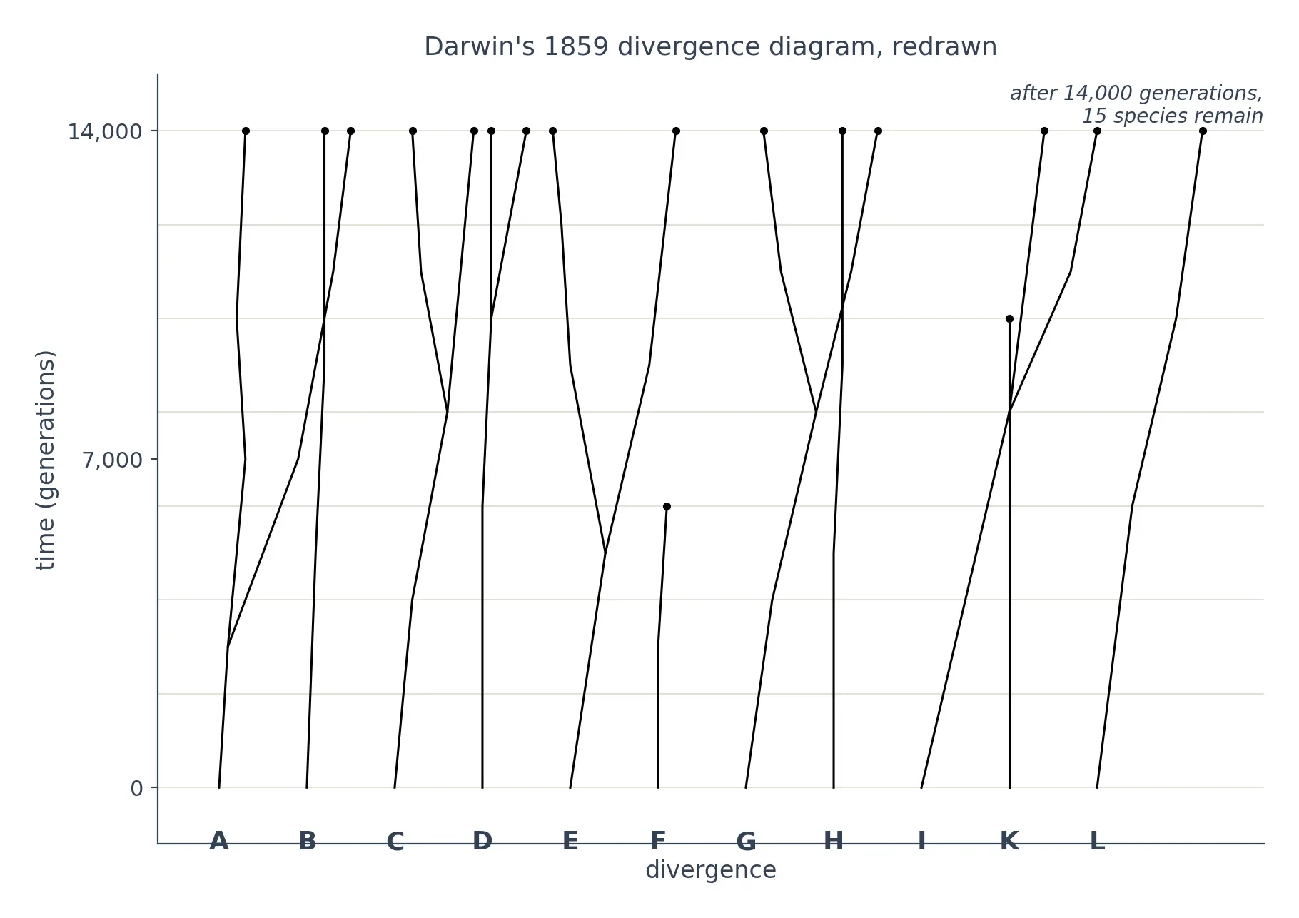
The diagram starts from 11 original species, labelled A to L, and follows them through time. The generations are horizontal lines, oldest at the bottom, and after 14,000 generations the diagram shows 15 species that differ to varying degrees from the originals. Some lines branch again and again. Some lines stop. Some species barely change at all.
The horizontal axis represents divergence between species. The vertical axis represents time across 14 time steps. Read that way, the diagram is a machine for thinking about splitting. Two lines that start close together can drift apart. One line can give rise to several. A line can end, and that ending is extinction, drawn as quietly as a branch that simply stops.
The main message is Darwin's principle of divergence, not simply common descent. Common descent says species share ancestors. Divergence says those descendants spread apart, filling different ways of life, until they differ enough to count as distinct species. That distinction matters, because it explains why one ancestor can produce a whole fan of forms. The tree of life, in Darwin's hands, was a picture of spreading out.
That spreading is driven by natural selection, the process explored in detail in our guide to natural selection. Selection favours different variants in different conditions, and over thousands of generations those small differences accumulate. The diagram lets you watch that accumulation without a single fossil or finch in view. It is abstract on purpose, so the pattern stands out.
"The affinities of all the beings of the same class have sometimes been represented by a great tree. I believe this simile largely speaks the truth." — Charles Darwin, On the Origin of Species (1859), Chapter 4
Darwin's sentence is careful. He says the simile "largely" speaks the truth. He does not say it speaks the whole truth. That caution runs through the whole book, and it runs through the tree of life ever since. A tree is a model of history, and models can be wrong in their details while getting the shape right.
1.3 The 1837 "I think" sketch and the coral doubt
The 1859 diagram did not come from nowhere. In 1837, in his Notebook B, Darwin sketched a small branching tree and wrote "I think" above it. He wrote that organised beings represent a tree, irregularly branched, with as many terminal buds dying as new ones generated. He was 28 years old, back from the Beagle voyage, and trying to hold a new idea in a few lines of ink.
That sketch is often reproduced as the birth of the tree of life. It is a birth, but it was a hesitant one. Darwin himself doubted the tree metaphor. In his notebooks he wrote: "The tree of life should perhaps be called the coral of life, base of branches dead; so that passages cannot be seen." A coral grows by adding living tips to a dead base. A tree, in the usual picture, has a living trunk that carries the whole history upward. Darwin saw the problem. Most of life's history is dead. The living species are only the tips. The passages between them — the extinct ancestors that connect one branch to another — cannot be seen directly. They have to be inferred.
That doubt was honest, and it still shapes the science. Every version of the tree of life is drawn from survivors. Darwin knew he was drawing a map with most of the roads erased: the living tree shows only the survivors, and the dead branches outnumber them vastly. He drew it anyway, because the roads that remain still point the way.
The coral image also explains why the tree of life is still being redrawn. New fossils fill in dead branches. New DNA sequences split old branches and join others. The trunk does not change its nature, but the shape of the crown keeps shifting as more tips are sampled. Darwin's diagram was a hypothesis in picture form, and a hypothesis is meant to be tested.
2. What the Tree of Life Actually Is
2.1 Nodes, branches, tips and the root — the anatomy in plain language
A phylogenetic tree is a diagram depicting the hypothesised degrees of evolutionary relationship among a selected set of taxa. That careful wording matters. A tree is a hypothesis, not a photograph of the past. It says: given the evidence we have, this is the best account of who is related to whom.
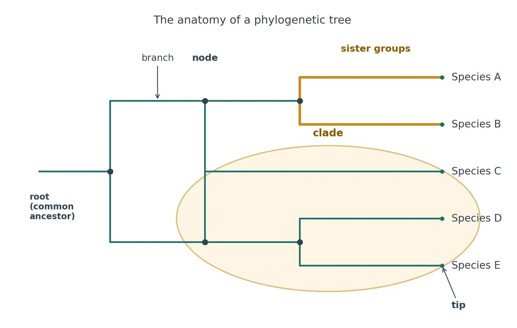
Start with the parts. The tips, also called terminal taxa, are the species or groups at the ends of the branches. They are the living or sampled organisms on the tree. The branches are the lines that connect them. Each node, the point where branches meet, represents a common ancestor shared by two or more terminal taxa. The root is the deepest node, the common ancestor of everything on the tree.
Think of a family reunion drawn as a diagram. You and your cousin meet at your shared grandparents. That meeting point is a node. Your grandparents and their siblings meet further back, at a deeper node. Keep going back and you reach the root of that family. A tree of life works the same way, except the family is all of life and the reunion stretches back billions of years.
Relatedness is read from the nodes, not from how far apart two tips sit on the page. More closely related taxa are connected by shallower nodes, nearer the tips. More distantly related taxa are connected by deeper nodes. Two species can sit side by side on a page and still be distant cousins, if their shared node lies deep in the tree. Two species drawn far apart can be close relatives, if their branches meet at a shallow node just below the tips.
2.2 Clades: the only groups that count
A clade, from the Greek klados, meaning branch, is a group composed of a common ancestor and all of its descendants. It is also called a monophyletic group. The term "clade" was coined in 1957 by biologist Julian Huxley, but the idea is older than the word. A clade is one node plus everything descending from it. Cut a branch at one point and take everything above the cut, and you have a clade.
Clades are nested inside one another, like boxes inside boxes. Mammals form a clade. Inside mammals, primates form a clade. Inside primates, apes form a clade. Inside apes, the great apes form a clade. Each smaller clade sits inside a larger one, because each ancestor sits inside the history of its own ancestors. That nesting is what makes the tree of life so useful. Once you know where a species sits, you know which larger groups it belongs to, and you can predict a great deal about it.
The test for a clade is simple: one cut. If you can separate a group from the rest of the tree with a single cut across one branch, and that group contains an ancestor and all of its descendants, it is a clade. If a group leaves some descendants out, or pulls in species from different branches, it fails the test. That test is the backbone of modern classification, and of the tree of life, and it is why some familiar names no longer count as proper groups.
2.3 What a tree is — and what it is not
The tree of life is a map of relationships, not a ladder. That is the sentence I would put on a classroom wall, because the ladder picture is the most stubborn wrong idea in evolution. A ladder has rungs, with one step above another and a top to reach. A tree has branches, and no branch is above another in value. Humans are not the top rung. Bacteria are not the bottom rung. Every living species sits at a tip, and every tip has been evolving for exactly as long as every other tip.
I disagree, plainly, with the idea that evolution is a march of progress from simple to complex to human. It is wrong, and the tree of life shows why it is wrong. A bacterium alive today is not a leftover from an early stage. It is the product of billions of years of evolution, just as you are. Its lineage has survived every extinction, every climate swing, every change of chemistry that the human lineage survived, and it has done so without becoming human. That is not failure. That is success on its own branch.
The tree of life is also not a timeline by itself. Branch length can mean different things, and on some trees it means nothing at all. A tree without a scale tells you who is related to whom, but not when the splits happened. To add dates, scientists need fossils, molecular clocks, and other evidence laid on top of the branching pattern. The branching pattern comes first. The dates come second.
The tree of life is a hypothesis of the evolutionary past, not a confirmed record. As OpenStax puts it, one cannot go back to confirm the proposed relationships. That sounds like a weakness, but it is the opposite. A hypothesis can be tested. New data can support it, revise it, or overturn it. The tree of life has survived more than a century and a half of testing, and it has changed shape many times in the process. That is how science is supposed to work.
The split at each node is a speciation event: one lineage becoming two. Our guide to speciation explains how that splitting happens in populations. Keep that link in mind as you read on, because every node on every tree in this article is a speciation event, drawn as a point.
Group type | Definition | The one-cut test | Example |
|---|---|---|---|
Monophyletic (a clade) | An ancestor plus all of its descendants | One cut separates the whole group cleanly | Mammals: the first mammal and every descendant, living and extinct |
Paraphyletic | An ancestor plus some, but not all, of its descendants | One cut leaves some descendants outside the group | Reptiles in the old sense: the ancestor of reptiles, birds, and crocodiles, but with birds left out |
Polyphyletic | Species from different branches grouped together, without their shared ancestor | No single cut can separate the group; it takes two or more cuts | Warm-blooded animals as a group: birds and mammals grouped by warmth, though their shared ancestor was cold-blooded |
Table 1: Monophyletic, paraphyletic, and polyphyletic groups compared. Only a monophyletic group — a clade — counts as a proper group in modern classification, because only it contains an ancestor and all of its descendants.
The reptile example in the table deserves a pause. In everyday language, reptiles are lizards, snakes, turtles, and crocodiles, and birds are something else. On the tree, birds sit inside the reptile branch. They descend from the same ancestor as crocodiles, and they are more closely related to crocodiles than crocodiles are to lizards. The old group "reptiles" left birds out, so it was paraphyletic. Modern classification either includes birds inside the reptile clade or stops using "reptiles" as a formal group. That is not wordplay. It is the tree correcting a name.
3. How to Read a Phylogenetic Tree
3.1 Follow the nodes, not the tips
The single rule that replaces most tree-reading confusion is this: the way species are connected through nodes as you travel away from the root is the only aspect of a tree that matters. Tip order, tip distance, and the length of the lines on the page are all secondary. The nodes carry the information.
To find how closely related two species are on the tree of life, trace their branches back until the branches meet. That meeting point is their most recent common ancestor. The pair whose shared node lies closer to the tips is more closely related. The pair whose shared node lies deeper is more distantly related. That is all there is to it, and it works on every tree, from a three-species diagram in a textbook to a tree of millions of species on a screen.
Try it with a simple picture in your head. Species A and B share a node just below the tips. Species C joins them at a deeper node. A and B are closer relatives than either is to C, even if C happens to be drawn right next to B on the page. The drawing can mislead your eye. The nodes do not lie.
3.2 Rotating branches changes nothing
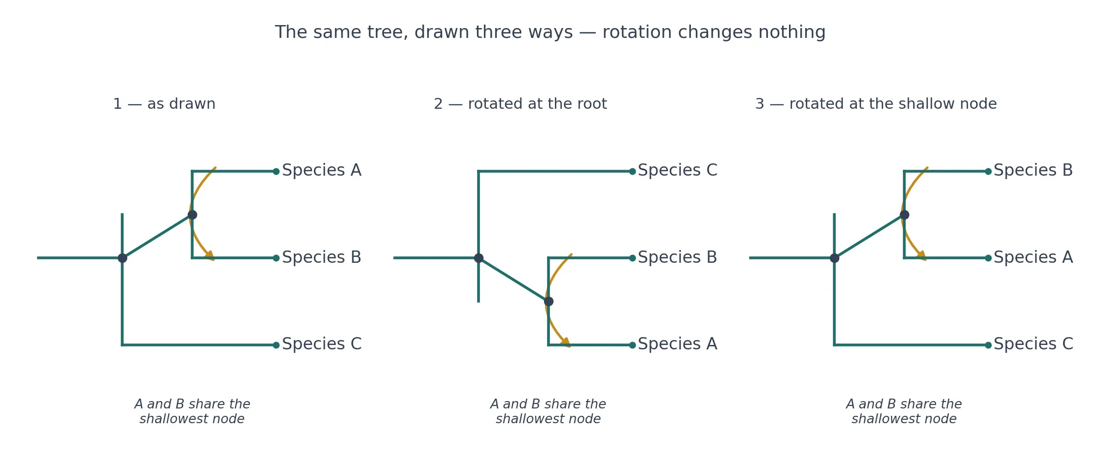
Branches may be rotated about nodes without any change in the relationships depicted. Three differently drawn trees can depict the exact same relationships among the same taxa. That sounds strange until you picture a mobile hanging from a ceiling. Spin one arm of the mobile and the ornaments swap sides, but the strings still connect the same ornaments to the same arm. A tree is the same. Rotating a branch flips which tip sits on the left and which sits on the right, and nothing about relatedness changes.
This is the most useful fact in this whole section, because it defeats the eye's habit of reading left to right. A common reading mistake is to treat tip order as meaningful. Switching the labels of two sister taxa produces a topologically equivalent tree, and the leftmost tip is not the oldest or most primitive. There is no oldest tip. There is no most primitive tip. All tips are the present day.
Trees can also be drawn in many orientations — vertical, sideways, circular — and still say the same thing. Darwin's Origin diagram grows upward. Many modern trees grow sideways, with the root on the left and the tips on the right. Circular trees put the root in the centre and the tips around the rim. The orientation is a design choice, not a claim about nature. Learn to read the nodes, and the orientation stops mattering.
3.3 Sister groups and the most recent common ancestor
Sister taxa, or sister groups, are pairs of terminal taxa or clades that branch from a common node and are considered closely related. If two branches share a node and nothing else shares that node, they are sisters. A species can have only one sister group at a given node, though that sister group can itself be a large clade.
The most recent common ancestor of two taxa is the point in the tree where their branches meet. That ancestor was a real organism, or a real population, that lived at a real time. It was not half one species and half another. It was its own thing, and its descendants went in two directions. Humans and chimpanzees, for example, share a common ancestor that lived 4.7 to 8.7 million years ago (about 6 million years is the commonly quoted midpoint), and that ancestor was neither a human nor a chimpanzee. It was the starting point for both lines.
When you read a tree, name the most recent common ancestor first, then ask what else descends from it. That habit keeps you honest. It stops you from saying one living species gave rise to another, because no living species sits at a node. Nodes are ancestors. Tips are descendants. A living species is never the ancestor of another living species.
3.4 Branch lengths: cladograms vs phylograms
Branch lengths mean different things on different trees. On a cladogram, they carry no time or change information. The branches are drawn only to show the branching pattern, and their lengths are chosen for readability. On a phylogram, branch lengths are proportional to evolutionary change or time. Longer branches mean more change, or more time, depending on the scale.
Always read the figure legend and scale before inferring anything from length. That is not fussy advice. It is the difference between a correct reading and a confident error. A long branch on a cladogram means nothing. A long branch on a phylogram can mean a lineage that changed fast, or one that split long ago, or both. The legend tells you which.
A useful analogy is a road map. A cladogram is like a diagram of which towns connect to which, with no distances marked. A phylogram is like a road map with a scale bar, where the length of the road tells you how far apart the towns sit. Both maps are useful. Neither is useful if you read it as the other kind.
3.5 Polytomies, outgroups and rooting
A polytomy is a node where more than two branches meet at once. It looks like a fork with three or more prongs. A polytomy usually means the data cannot yet resolve the order of the splits, not that three species split in the same instant. It is a mark of uncertainty, drawn honestly. As more data arrives, polytomies often resolve into a series of two-way splits. Some stay unresolved, because the splits happened so close together in time that little evidence survives to order them.
An outgroup is a lineage outside the group under study, used to root the tree. Pick a species you know sits outside the group, place it at the base, and the root falls into place. The outgroup gives the tree its direction: without it, you know who is related to whom, but not which direction time runs. Rooting is the step that turns an unrooted network into a tree with a past and a present.
That rooting step matters more than it looks. Move the root and the story changes. A group that looked like a single early branch can turn out to be a late offshoot, and a species that looked primitive can turn out to be highly specialised. Good trees state their outgroup and their rooting method, so a reader can judge the choice.
3.6 A worked example: read a primate tree step by step
Put the rules together on a small primate tree. Picture four tips: human, chimpanzee, gorilla, and orangutan. The tree shows humans and chimpanzees sharing a shallow node. That node joins a deeper node shared with gorillas. That larger group joins orangutans at a still deeper node. Read by nodes, the story is plain. Humans and chimpanzees are sister taxa. Gorillas are the next closest relatives of the human-chimpanzee pair. Orangutans branched off earlier than the gorilla split.
Now rotate the human and chimpanzee branches. The picture flips, but the relationships do not change. Now draw the tree sideways, root on the left, tips on the right. The picture looks different, but the nodes are the same. Now check the branch lengths. If this is a cladogram, the lengths mean nothing. If it is a phylogram with a time scale, the human-chimpanzee node sits at 4.7 to 8.7 million years ago (about 6 million years as the commonly quoted midpoint), and the deeper nodes sit further back. The legend decides.
The same reading works on any tree you meet, and the speciation events behind each node are explained in our guide to speciation. Find the shallowest shared node, name the most recent common ancestor, and ignore the left-to-right order. That is the whole skill, and it is enough to read a tree of life in a textbook, a paper, or a museum display.
If you are studying for AP Biology: the vocabulary box
Node: a branching point on a tree; the most recent common ancestor of the taxa above it.
Root: the deepest node; the common ancestor of all taxa on the tree.
Outgroup: a lineage from outside the group under study, used to root the tree.
Sister taxa: two taxa or clades that share a node and are each other's closest relatives on the tree.
Synapomorphy: a shared derived character, inherited from a common ancestor, that marks a clade. Only shared derived characters establish relationships; shared ancestral characters are too widespread and unique traits too restricted to tell us about relationships within a group.
Parsimony: the principle of preferring the tree that requires the fewest evolutionary changes to explain the data.
Trees are testable hypotheses, not facts carved in stone. Phylogenetic trees and cladograms are graphical representations of evolutionary history that can be tested, and they are constantly revised as new evidence arrives. A tree that cannot change is not science. A tree that does change, when the evidence demands it, is science working as it should.
The 5-step reading checklist
Find the root first, so you know which direction time runs.
Trace two species back to their most recent shared node; the shallower the node, the closer the relationship.
Ignore tip order and tip distance; only the nodes decide relatedness.
Check the legend before reading branch length; on a cladogram it means nothing, on a phylogram it means change or time.
Look for the outgroup, the support values, and any polytomies, so you know where the tree is certain and where it is not.
4. From Linnaeus to Darwin to Haeckel: Before DNA
4.1 Linnaeus: naming without history
Carl Linnaeus gave biology its naming system a century before Darwin gave it a history. His Systema Naturae was first published in 1735, and the 10th edition of 1758 is the starting point of zoological nomenclature and the first work to consistently apply binomial nomenclature across the animal kingdom. Every species got two Latin names, a genus and a species, and every species got a place in a ranked system of classes, orders, genera, and species.
The scale of that 10th edition is worth picturing. It listed about 10,000 species in total — about 6,000 plants and 4,236 animals — and divided the animal kingdom into six classes: Mammalia, Aves, Amphibia, Pisces, Insecta, and Vermes. Ten thousand species sounds small now, when millions are known, but in 1758 it was an attempt to name the whole living world in one book.
Linnaeus also made calls that still look sharp today. In the 10th edition, whales and manatees were moved from the fishes into the mammal class, and bats were removed from the birds and classified as mammals. He grouped by anatomy, not by habitat or by how an animal moved. A whale swims like a fish, but it breathes air, gives live birth, and nurses its young. A bat flies like a bird, but it has fur, gives live birth, and nurses its young. Linnaeus saw past the surface.
Taxonomy and phylogeny are related but different jobs. Taxonomy names and ranks organisms. Phylogeny reconstructs their history. Linnaeus did the first job brilliantly, without the second. His system had no time in it. Species sat in boxes, and the boxes sat in larger boxes, but nothing said how the boxes came to be. That missing history was the gap Darwin would fill, and the gap that later tree-builders would spend a century and a half closing. Our guide to animal classification covers the naming system in full; this article is about the history behind the names.
4.2 Darwin: history without a mechanism for inheritance
Darwin supplied the history that Linnaeus lacked, but he did so without a working theory of inheritance. He knew offspring resemble parents. He did not know how traits are passed on, or why they sometimes skip a generation, or how new variation arises. Genetics would arrive decades later, with Mendel rediscovered and DNA identified as the carrier of heredity in the twentieth century.
That gap did not stop the tree of life from working. Darwin's argument ran on variation, selection, and time, and those three were enough to explain branching. Species split when populations diverged under different conditions. The splits accumulated into a tree. The mechanism of inheritance could wait, because the pattern of descent was visible in anatomy, in fossils, and in the geographical distribution of species.
It is worth remembering how much Darwin did with how little. He had no DNA, no molecular clock, no computers, and no fossil record as complete as the one we have now. He had a diagram, a theory, and a mass of observations. The tree of life he drew was a sketch of a process, and the process turned out to be right even though the details of inheritance were still unknown.
4.3 Haeckel 1866: the first tree of all life — and its ladder problem
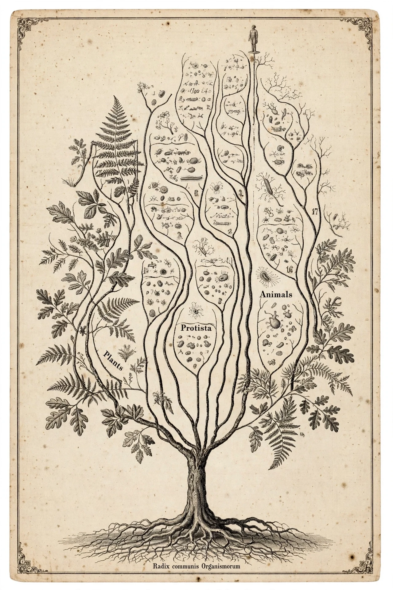
Ernst Haeckel published the first Darwinian phylogenetic tree of life in his Generelle Morphologie der Organismen (1866), showing three kingdoms — animals, plants, and Protista — arising from a common root he called Moneren. It was the first attempt to draw the whole of life as one tree, and it set the shape of the idea for generations. Haeckel also coined the term "phylogeny", the evolutionary history of organisms, in the same 1866 work, and defined it there.
Haeckel's trees were beautiful, branching, and full of life. They were also shaped by a bias he did not hide. His famous "Pedigree of Man" of 1874 placed humans at the very top of the tree, above the apes. Modern biologists read that layout as a hierarchy Haeckel imposed, not a finding, since nothing in the evidence makes humans the goal of evolution. The tree of life was drawn as a ladder with a crown, and the crown was us.
That ladder problem is not a small footnote. A tree with humans at the top tells a story about progress, with simpler forms below and higher forms above. The evidence tells a different story: a branching bush, with every living tip at the same height in time. Haeckel's drawing is a historical document, and it should be read as one. It shows how a powerful idea can be bent by the assumptions of its time, and how later evidence straightens it out.
4.4 Hennig and cladistics: grouping by shared derived characters
The fix for Haeckel's ladder came from a German entomologist named Willi Hennig. His cladistics, set out in Grundzüge einer Theorie der phylogenetischen Systematik in 1950 and in English as Phylogenetic Systematics in 1966, made shared derived characters — synapomorphies — the sole source of phylogenetic evidence, and grouping by synapomorphy the basis of clades.
The rule is strict, and its strictness is its strength. A shared derived character is a feature that evolved in the common ancestor of a group and is passed to its descendants. Feathers mark birds, because feathers evolved in the bird lineage. Hair marks mammals, because hair evolved in the mammal lineage. A shared ancestral character, by contrast, is too widespread to mark a group. Backbones mark vertebrates, but they cannot tell you which vertebrates are closest to each other, because all vertebrates have them. A unique trait marks one species only, and tells you nothing about its relatives.
Hennig's rule turned tree-building from an art into a testable method. Group species by the derived characters they share, and the groups that emerge are clades. Ignore the rule, group by overall similarity or by habit, and you get paraphyly, polyphyly, and ladders with humans at the top. Cladistics did not finish the job — DNA would later transform it — but it gave the job its logic. Every modern tree, whether built from bones or from base pairs, still runs on Hennig's question: which characters are shared because they were inherited from a common ancestor?
5. The Molecular Revolution: Woese and the Three Domains
5.1 Why anatomy hit a wall with microbes
Anatomy works well on animals and plants. A bird has feathers, a mammal has hair, a flowering plant has flowers, and those features mark their groups cleanly. Anatomy hits a wall with microbes. A bacterium is a single cell, a few micrometres long, with no feathers, no hair, no flowers, and few visible features to compare. Two microbes can look identical under a microscope and be as different from each other as a mushroom is from a whale. Two microbes can look different and be close cousins. The eye cannot tell.
That wall mattered, because microbes are most of life. They run the planet's chemistry, they live in boiling springs and Antarctic ice and deep rock, and they outnumber every animal and plant combined in both species and cells. A tree of life built on anatomy alone left its largest branches blank, or drew them as a single vague twig labelled "bacteria". The tree needed a new kind of character, one that microbes carry in abundance and that changes slowly enough to read across billions of years.
The answer was already inside every cell. It was a molecule that every living thing shares, that does the same job in all of them, and that changes slowly enough to keep a record of deep time.
5.2 16S rRNA: a molecule that keeps time
That molecule is 16S ribosomal RNA. Ribosomes are the machines that build proteins, and they exist in every cell. The gene for 16S rRNA, the RNA component of the small ribosomal subunit in prokaryotes, is universal and changes slowly. Because it changes slowly, its sequence differences measure time since divergence. Two species that split recently have nearly identical 16S sequences. Two species that split billions of years ago have sequences that differ at many positions.
Carl Woese used that gene as a molecular clock. He did not compare whole genomes — the technology did not exist yet. He compared fragments of ribosomal RNA, cataloguing the short sequences, or oligonucleotides, that each microbe carried. The method was slow, painstaking work, done by hand and by early computing, and it required patience that few other researchers had. Woese had it.
I remember first learning about Woese in a microbiology lecture, and the lecturer put it simply: Woese stopped looking at what microbes look like and started reading what they are made of. That sentence stayed with me, because it captures the shift. Anatomy asks what a creature looks like. Molecules ask what it inherited. For microbes, the second question is the only one that works.
5.3 1977: a third domain nobody expected
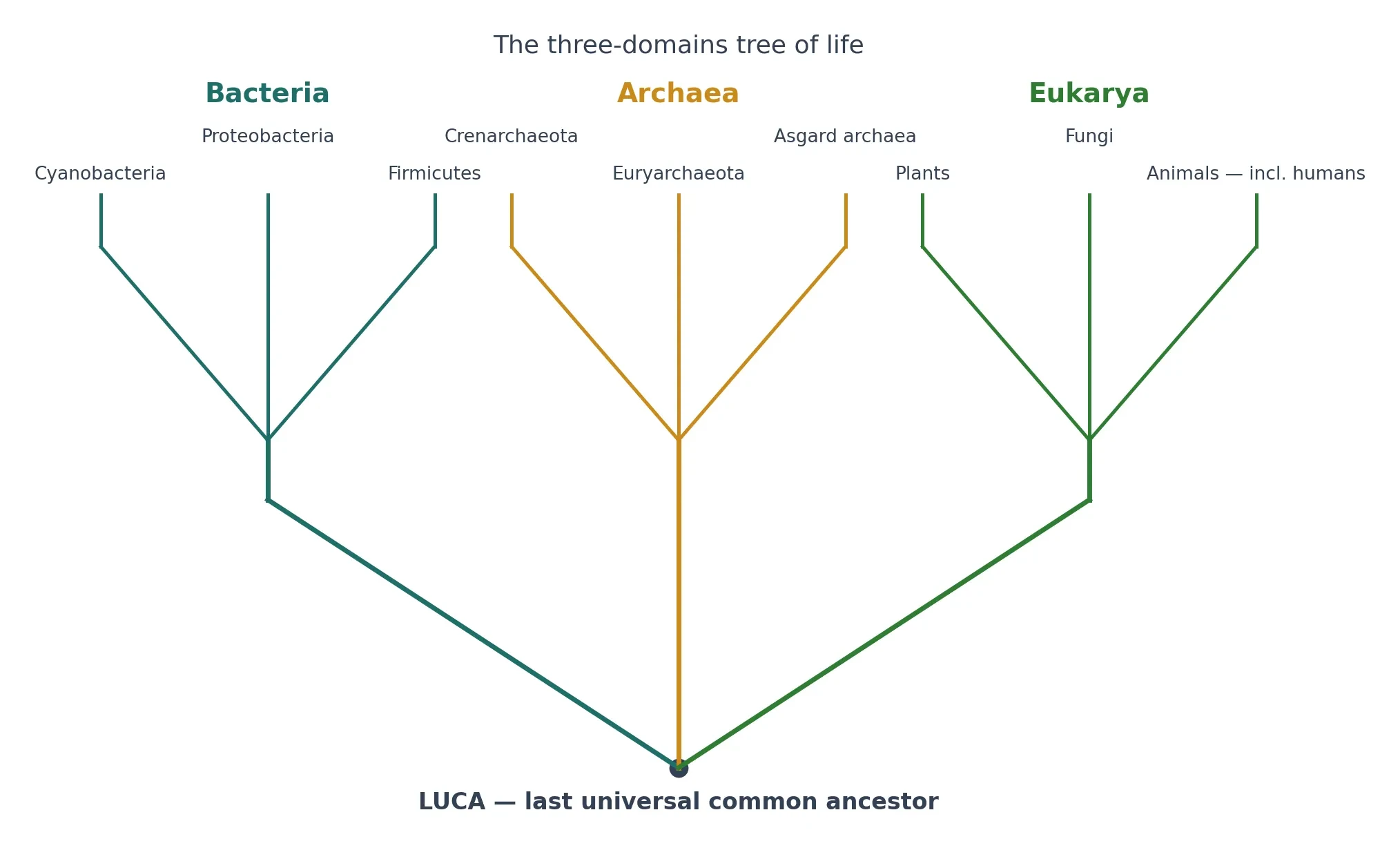
In 1977, Carl Woese and George Fox showed by 16S ribosomal RNA sequence analysis that methanogenic microbes were as different from bacteria as from eukaryotes, revealing a third primary line of descent — the "archaebacteria", now Archaea. The methanogens, microbes that make methane in oxygen-free places, were not odd bacteria. They were something else entirely, a branch as deep as the split between bacteria and eukaryotes.
The paper's abstract states the finding in one sentence, and the sentence is worth reading exactly as Woese and Fox wrote it.
"A phylogenetic analysis based upon ribosomal RNA sequence characterization reveals that living systems represent one of three aboriginal lines of descent: (i) the eubacteria, comprising all typical bacteria; (ii) the archaebacteria, containing methanogenic bacteria; and (iii) the urkaryotes, now represented in the cytoplasmic component of eukaryotic cells." — Carl Woese and George Fox, Proceedings of the National Academy of Sciences USA (1977)
Three lines, not two. Not plants and animals, not prokaryotes and eukaryotes, but three aboriginal lines of descent. The word "aboriginal" is doing heavy work there. Woese was saying these lines go back to the beginning, to the earliest splits in the history of life. They are not branches off a main trunk. They are three trunks, or three roots from one root.
The reaction was not instant acceptance. Many microbiologists had spent careers sorting microbes by shape, by metabolism, by what they eat and where they live. A molecule was telling them their sorting was wrong at the deepest level. Woese's claim was argued over, tested, and eventually confirmed by more sequences, more genes, and more genomes. The third domain was real.
5.4 The shock of Archaea — and the 1990 three-domain system
Archaea resemble bacteria in cell structure. Both have no nucleus, and both are prokaryotes. That resemblance is why they were missed for so long. But their 16S rRNA and other fundamental genes differ from bacteria as much as from eukaryotes. Look at their chemistry and the difference deepens. Their cell membranes, their enzymes, and their information-processing machinery share features with eukaryotes that bacteria lack. They look like bacteria and read, in their genes, like something else.
Woese's discovery replaced the five-kingdom scheme with three equally distinct domains — Bacteria, Archaea, and Eukarya — formally proposed as the three-domain system in 1990, in a paper by Woese, Kandler, and Wheelis. The three-domain system is the framework this article uses from here on for the tree of life, and it is the framework most textbooks still teach. It puts humans, mushrooms, and oak trees together in Eukarya, one domain among three, and it puts the vast majority of life's diversity in the other two.
That framework may not be the last word. Recent phylogenomic analyses indicate eukaryotes likely emerged from within Archaea, specifically from the Asgard lineage — which, if confirmed, turns the three-domain tree into a two-domain tree. The story of that challenge belongs to a later section, where the Asgard evidence is laid out in full. For now, hold both ideas at once. The three-domain system was a revolution, and revolutions can themselves be revised. The tree of life did not stop moving in 1990. It never stops moving. That is not a failure of the science. It is the science.
6. Building a Tree, Step 1: Characters and Data
Every tree of life starts long before anyone draws a branch. It starts with a question that sounds simple and turns out to be anything but: what can we compare, fairly, across very different living things? A wing and a fin do not look comparable at first glance. A whale and a bat seem to belong in different worlds. Yet both pairs can sit on the same tree of life, because tree builders do not compare whole animals. They compare characters — single, heritable features that can be scored, one by one, across the species in the study.
A character can be almost anything that is inherited and varies. The shape of a tooth. The number of toes. The presence of feathers. The sequence of letters in a gene. Each character is a small piece of evidence. One character on its own proves almost nothing. Hundreds or thousands of them, lined up side by side, start to tell a story. That is the quiet, unglamorous foundation of the tree of life: not a grand theory, but a table of features, carefully chosen and honestly scored.
Get the characters wrong and everything that follows goes wrong too. A tree built from misleading characters will look confident and still be wrong. A tree built from good characters, even a modest number of them, can survive decades of new evidence. So before any method runs, before any software opens, a researcher has to decide what counts as evidence — and what does not.
6.1 Morphological characters: bones, teeth and embryos
For more than a century, the tree of life was built almost entirely from bodies. Morphological characters are features you can see, touch, measure and draw: the bones of a skull, the cusps on a molar, the pattern of veins in a leaf, the way an embryo folds in its first days. Palaeontologists still depend on them, because for extinct species a skeleton is often all that remains. A fossil jaw with a particular tooth pattern can place an animal on the tree of life millions of years after it died, when no DNA survives to help.
Morphology has a strength no gene can match: it connects the living to the dead. Fossils carry characters and dates together, so they anchor branches in real time. A fossil with feathers and a long bony tail does not just suggest a link between dinosaurs and birds; it shows what that link looked like, and roughly when it lived. That is why the fossil record still matters to tree building, even in an age of genomes. DNA can tell us that two groups are related. Only a fossil can show us the animal that stood at the fork in the road.
Morphology also has a weakness, and it is a serious one. Bodies are shaped by how an animal lives, not only by who its ancestors were. A dolphin and a shark both have streamlined bodies, fins and tails built for speed in water. Those features are real, and they are useful for swimming, but they say nothing about shared ancestry. Dolphins are mammals; sharks are fish. Their similar shapes are a response to the same environment, not a sign of a recent common ancestor. Any tree that treated a streamlined body as proof of kinship would put dolphins beside sharks — and be wrong.
Embryos help, because early development often preserves clues that adult bodies hide. Two animals that look nothing alike as adults may start from strikingly similar embryos, with the same pouches, arches and limb buds appearing in the same order. That shared developmental pattern is a character too, and often a more honest one than the adult form. Even so, morphology alone has limits. There are only so many bones to measure, and in some groups — above all the microbes — there are hardly any visible features at all.
6.2 Molecular characters: DNA, RNA and proteins
The molecular revolution changed the raw material of tree building. Instead of comparing bones, researchers compare sequences: the order of letters in DNA, the sequence of RNA, or the amino acids in a protein. Each position in a sequence is a character. A gene a thousand letters long gives a thousand characters at once. A whole genome gives millions. That scale is the first great advantage of molecular data. Comparing DNA, RNA or amino-acid sequences often provides large datasets that can resolve relationships morphology alone cannot (Knowt).
The second advantage is that molecular characters work where bodies fail. Bacteria and archaea have few visible features to compare, yet their genes differ in clear, measurable ways. That is how Carl Woese found a whole domain of life that anatomy had missed: the molecules carried a signal the microscope could not see. For microbes, for fungi, for tiny marine animals that all look like pale blobs, DNA is often the only workable evidence.
Molecular data also carry their own traps. A single letter in DNA can change back again, erasing the record of an earlier change. Two species can end up with the same letter at the same position by coincidence, not by shared ancestry — the molecular version of the dolphin and the shark. And genes do not always follow the same history as the species that carry them, a problem we will meet head-on in §10. A gene tree is not automatically a species tree. That distinction matters, and honest tree builders keep it in view from the start.
The practical lesson is simple: morphology and molecules are partners, not rivals. Morphology brings fossils, development and the shape of real bodies. Molecules bring volume, precision and access to the microbial majority of life. The strongest trees use both, and say so plainly when the two kinds of evidence disagree.
Feature | Morphological characters | Molecular characters |
|---|---|---|
What is compared | Bones, teeth, leaves, embryos, body plans | DNA, RNA and amino-acid sequences |
Number of characters | Dozens to hundreds per study | Thousands to millions per study |
Greatest strength | Works for fossils and extinct species; connects living and dead | Resolves relationships morphology alone cannot; works for microbes |
Greatest weakness | Similar lifestyles can produce similar bodies; few features in microbes | Letters can change back; genes can disagree with species history |
Examples | Feathered fossil dinosaurs, tooth cusp patterns, embryo limb buds | 16S rRNA sequences, whole genomes, protein sequences |
Best used for | Placing fossils, dating branches, testing body-based ideas | Deep microbial branches, closely related species, large datasets |
Table 2: Morphological vs molecular characters. Morphology anchors the tree of life in fossils and real bodies; molecules supply the volume and precision that anatomy cannot reach on its own.
6.3 Homology vs homoplasy: same look, different history
Here is the single most important distinction in all of tree building. Homologous characters are shared because of common ancestry. Homoplastic characters look similar because of convergent evolution, or because a feature was lost and then regained. Homology is evidence. Homoplasy is noise. Mistake one for the other and the tree of life bends in the wrong direction.
Homologous characters are shared because of common ancestry and are informative for trees; analogous characters look similar because of convergent evolution and mislead trees if mistaken for homology (Knowt). The forelimb of a human, a bat, a whale and a mole tells the story cleanly. A hand, a wing, a flipper and a digging paw look nothing alike and do completely different jobs. Yet inside each one sits the same plan: one upper-arm bone, two forearm bones, a cluster of wrist bones, and five digits. That shared plan is inherited from a common ancestor that had five digits. The jobs changed; the blueprint stayed.
The wings of a bat and a bird are the opposite case. Both are wings, both fly, and both are built from a forelimb — so they share a deep homology as forelimbs. But the wing itself, as a flying surface, evolved separately in bats and in birds. A bat wing is a membrane stretched across elongated fingers. A bird wing is feathers anchored to a fused hand. Treat "has wings" as a single character and you will group bats with birds, ignoring the much stronger evidence that bats belong with other mammals. That is the trap of convergent evolution: natural selection solves the same problem — flying, swimming, digging — with similar shapes in unrelated lineages, again and again.
Not every shared character is useful, even when it is genuinely homologous. Only synapomorphies — shared derived characters — can establish relationships. Shared ancestral characters, called plesiomorphies, are too widespread, and unique traits, called autapomorphies, are too restricted to tell us about relationships within a group (Gregory). Having a backbone is a real shared character, but it groups everything from lampreys to humans together and says nothing about which vertebrates are closest to each other. Having feathers, by contrast, is a shared derived character of birds: it marks the bird branch and no other. Having a single unusually long tail feather found in only one species marks that species alone. It is interesting, but it cannot group that species with anything else.
Good tree builders therefore spend a surprising amount of time throwing characters away. A character that is ambiguous, that varies within a species, or that cannot be scored the same way in every species in the study is worse than useless — it adds noise that can drown out the real signal. The discipline of character choice is what separates a careful tree from a pretty diagram.
6.4 Alignment: lining up evolution so positions can be compared
Molecular characters have one extra step that morphology does not, and it is the step where many trees quietly fail. Before two DNA sequences can be compared, they must be aligned — lined up so that position 1 in one species is compared with position 1 in the other, position 2 with position 2, and so on. That sounds mechanical. It is not. Genes gain and lose letters over time. A stretch of DNA that is 100 letters long in one species may be 103 in another, because three letters were inserted somewhere along the way. Where exactly did the insertion happen? The alignment has to decide, by inserting gaps into the shorter sequence at the right places.
All tree-building methods assume the alignment is correct; errors in the alignment can lead to a very misleading tree (Los Alamos National Laboratory HIV Database). A gap placed two positions too far to the left can make unrelated letters look like matches, and real matches look like differences. The software will still produce a tree. It will look just as confident as a tree built from a correct alignment. Nothing in the output will flash a warning. That is why experienced researchers inspect alignments by eye, especially in the messy regions where insertions and deletions pile up, and trim away the parts they cannot align with confidence.
The standard construction workflow makes the order clear: first sequence data collection, then sequence alignment and trimming, then model selection and fitting, then tree construction and evaluation (MDPI Genes). Alignment comes before the tree, not after it, and trimming — deliberately cutting out the unreliable columns — is part of the job, not a failure. A shorter alignment you trust beats a longer one you do not.
Think of alignment like lining up two copies of the same book after different editors have cut and pasted passages in different places. If you line up the chapters wrong, every comparison that follows is nonsense, however careful the later analysis. The tree of life is only as honest as the alignment beneath it. That is an unglamorous truth, and it is also the reason the best tree papers describe their alignments in detail instead of hiding them in a supplement nobody reads.
7. Building a Tree, Step 2: The Methods
Once the characters are chosen and the sequences are aligned, the real puzzle begins. There are usually far too many possible trees to check one by one. With ten species, the number of possible branching patterns already runs into the millions. Nobody finds the best tree by trying them all. Instead, scientists use methods: rules for scoring trees, searching among them, and deciding which one deserves to be drawn.
The two main categories of tree inference are distance-based methods, which first convert data into a matrix of pairwise evolutionary distances and then build a tree from it, and character-based methods, which use the individual substitutions in the alignment (MDPI Genes). Distance methods compress the data into a summary — how far apart is every pair of species? — and then build from that summary. Character-based methods keep the detail, asking at every position in the alignment what each tree would require. The summary is faster. The detail is richer. Neither is right for every job, and in practice researchers use several methods and look for agreement (Fiveable).
I remember the first time I watched a tree being built from real data, sitting beside a colleague who had spent months collecting sequences from a group of unassuming soil fungi. She clicked a button, and the screen filled with a branching diagram that looked, to my untrained eye, like a finished answer. She laughed and clicked again. A different method gave a slightly different tree. A third method moved one whole branch to the other side. "Which one is right?" I asked. She shrugged in the way only someone who truly understands a method can shrug. "That," she said, "is the whole job." The tree of life is not printed by a machine. It is argued for, method by method, until the evidence converges — or until the disagreement itself becomes the finding.
7.1 Maximum parsimony: the simplest tree wins
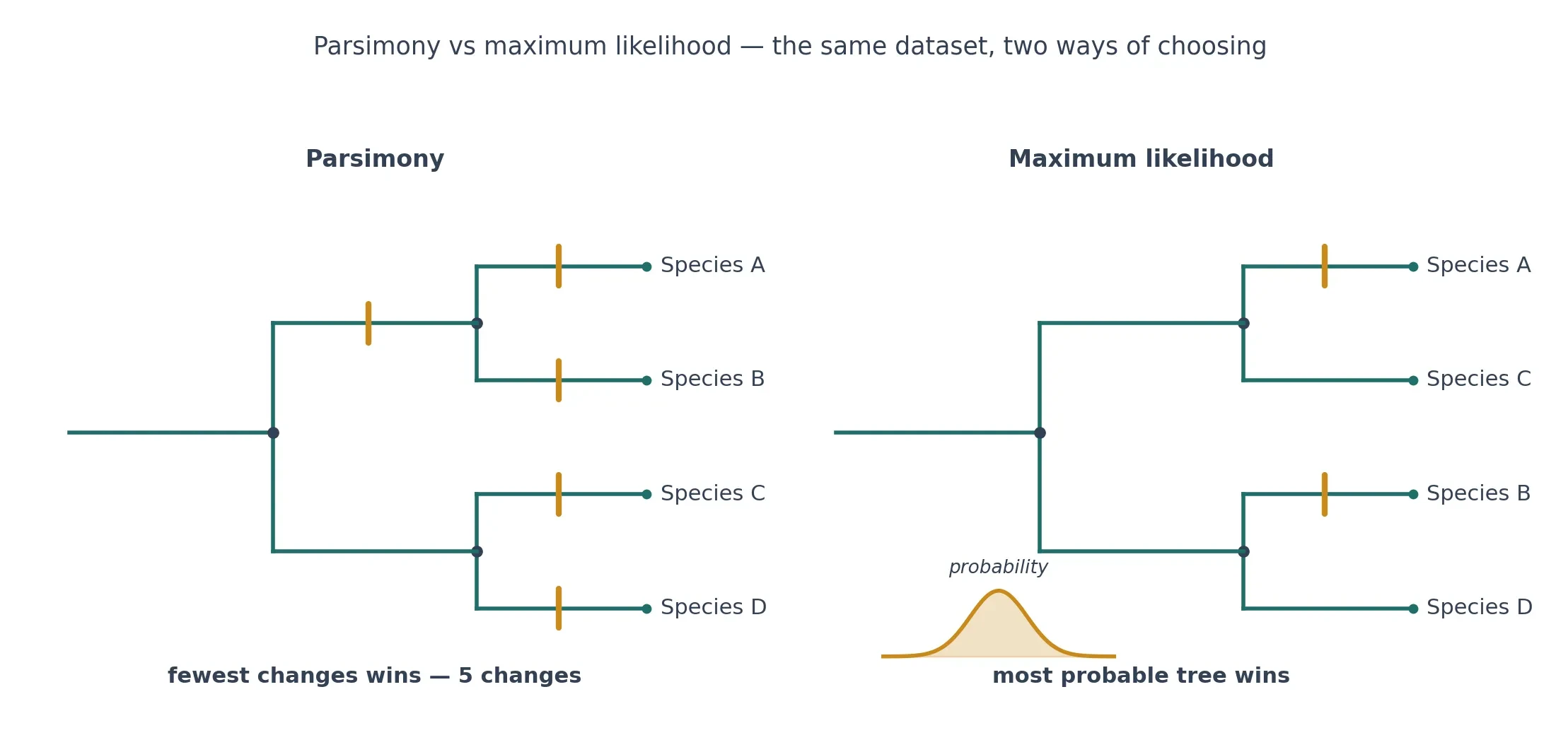
Maximum parsimony is the oldest idea in the modern toolkit, and the easiest to explain at a dinner table. It seeks the tree requiring the fewest evolutionary changes to explain the observed data — Occam's razor applied to trees (MDPI Genes). If two trees both explain your data, but one needs twelve changes and the other needs twenty, parsimony picks the twelve-change tree. The logic is that evolution, while messy, does not usually take the long way round when a short path will do.
Imagine four species and a single DNA position. Three species have the letter A there; one has the letter T. A tree that groups the three A species together needs one change, A to T, on the branch leading to the odd one out. A tree that scatters the A species across different branches needs several independent changes. Parsimony picks the first tree. Multiply that judgement across thousands of positions, and the tree with the lowest total number of changes wins.
That simplicity is also its weakness. Parsimony counts every change as equal, and evolution does not. Worse, parsimony can be fooled when two branches have both evolved very fast. Two fast-evolving lineages will each have accumulated many changes, and by chance some of those changes will match. Parsimony sees those coincidental matches, counts them as shared ancestry, and pulls the two long branches together into a false grouping. This is long-branch attraction, and it is parsimony's best-known failure. It is also why parsimony alone is rarely trusted for deep, ancient branches, where fast evolution and long times make coincidental matches common.
7.2 Distance methods: neighbour-joining and the distance matrix
Distance methods take a different shortcut. First, they measure how different every pair of species is — a distance matrix, a table with a number for each pair. Then they build a tree that fits those distances as closely as possible. The detail of individual characters is gone; what remains is a set of pairwise summaries. The gain is speed. The loss is information. Two species can be the same distance apart for very different reasons, and the matrix cannot tell you which.
The best-known distance method is neighbour-joining, created by Naruya Saitou and Masatoshi Nei in 1987. It starts from a star tree, with all species radiating from a single centre, and repeatedly joins the pair of taxa that minimises total branch length (Saitou and Nei). It is quick, it always finishes, and it always produces a single tree. Distance methods always produce a single tree, while parsimony and likelihood methods evaluate many hypothetical trees before choosing the best (MDPI Genes).
That single-tree certainty can mislead a newcomer. A neighbour-joining tree is a best fit to the distances, not a verdict. If the distances are noisy — and they often are, when sequences are short or saturated with repeated changes — the tree will be confidently wrong. Neighbour-joining is at its best as a first look: a fast sketch of the data, a way to spot odd sequences or mislabelled samples before the slower methods run. Many published trees still start life as a neighbour-joining sketch. Few end there.
7.3 Maximum likelihood: which tree makes the data most probable
Maximum likelihood asks a subtler question than parsimony. Instead of counting changes, it asks: given this tree, and given a model of how DNA changes, how probable is the data we actually see? The tree that makes the observed sequences most probable wins. A tree that requires an unlikely pattern of changes scores badly, even if it needs few changes in total.
The method was founded for DNA sequences by Joseph Felsenstein's 1981 paper, "Evolutionary trees from DNA sequences: a maximum likelihood approach", which showed how to calculate the probability of aligned sequences given a tree. It is the second most cited paper in that journal, with over 9,000 citations (Journal of Molecular Evolution retrospective). Felsenstein's insight was to treat tree building as a problem in probability, not just in counting. That shift still shapes the field.
In most comparative studies, maximum likelihood yields the best trees, but it is very computationally intensive and was historically almost unusable with more than a few dozen sequences (Los Alamos National Laboratory HIV Database). Calculating the probability of the data for a single tree is already demanding. Doing it for thousands of candidate trees is a serious computing job. Modern software has pushed the practical limit from dozens of species to thousands, but likelihood remains the slow, careful method — the one researchers turn to when the answer matters and the computer time is worth spending.
Likelihood also has a quiet advantage: because it uses an explicit model, its assumptions are out in the open, where they can be examined and improved. Parsimony hides its assumptions; likelihood declares them. That transparency is a large part of why likelihood became the workhorse of modern phylogenetics.
7.4 Bayesian inference: a forest of probable trees
Bayesian inference takes one more step back from the idea of a single best tree. Instead of asking which tree is best, it asks: given the data, the model, and what we knew before, how probable is each tree? It uses Bayesian probability theory to estimate the posterior probability distribution of trees, employing Markov Chain Monte Carlo algorithms to sample from that distribution (Fiveable).
The sampling is the key. A Bayesian analysis does not return one tree. It returns a forest — thousands of trees, sampled in proportion to how well each one fits the data. Trees that fit well appear often in the sample. Trees that fit badly appear rarely or not at all. The result is usually drawn as a single consensus tree, with each branch labelled by the fraction of sampled trees that contain it. That fraction is the posterior probability: a direct statement of confidence, in a form a reader can grasp at a glance.
This is powerful, and it is easy to misread. A posterior probability of 0.98 sounds like near-certainty, and in a well-behaved analysis it is strong support. But posterior probabilities depend on the model and on the prior assumptions fed into the analysis, and they can be overconfident when the model is wrong. Bayesian trees also take time: the sampling chain must run long enough to explore the forest properly. Used well, Bayesian inference gives the richest picture of uncertainty in the field. Used carelessly, it gives a beautiful tree with confidence values that flatter the data.
7.5 Substitution models in plain language (why all changes are not equal)
Every likelihood and Bayesian analysis rests on a substitution model: a set of rules about how DNA letters change over time. The simplest model says all changes are equally likely — A to T is as probable as A to G, and every position changes at the same rate. Real DNA does not behave that way. Some changes are chemically easy and happen often. Others are rare. Some positions in a gene are free to change, while others are so important to the protein that almost any change is fatal and never survives.
A realistic model therefore makes distinctions. It may allow transitions — swaps between the two similar bases, A with G, or C with T — to happen more often than transversions, swaps between the two different kinds. It may let different positions evolve at different speeds, so that a fast-changing third position in a codon is not treated like a slow-changing first position. It may allow the four letters to appear with unequal frequencies, because real genomes are often rich in A and T, or rich in G and C.
Choosing the right model matters, which is why model selection is a named step in the standard workflow, between alignment and tree construction (MDPI Genes). A model that is too simple will be fooled by repeated changes it did not expect. A model that is too complex will chase noise. Researchers test several models against their data and pick the one that fits best without overfitting.
The underlying logic reaches back to neutral theory, the idea that much molecular change is driven by chance rather than by selection. That is the framework explored in the companion article on genetic drift, and it is what makes substitution rates steady enough to use as clocks — the subject of the molecular clock article. A tree method that ignores how DNA actually changes is like a mapmaker who ignores the terrain. The model is the terrain. Get it roughly right, and the tree of life that follows has a chance of being right too.
Method | Core idea | Key assumption | Strength | Weakness | Speed |
|---|---|---|---|---|---|
Maximum parsimony | Fewest evolutionary changes wins | All changes equally likely; simplest is best | Simple, transparent, needs no model | Fooled by long-branch attraction; ignores rates | Fast on small datasets |
Distance (neighbour-joining) | Build from a matrix of pairwise distances | Distances capture the true history | Very fast; always gives one tree | Throws away character detail; noise in distances misleads | Very fast |
Maximum likelihood | Tree that makes the data most probable wins | Substitution model is roughly right | Best trees in most comparisons; assumptions explicit | Computationally intensive; slow on huge datasets | Slow |
Bayesian inference | Sample trees in proportion to their probability | Model and priors are reasonable | Direct confidence values; shows uncertainty honestly | Can be overconfident if the model is wrong; needs long runs | Slow |
Table 3: The four tree-building methods compared. No single method wins every time, which is why careful studies run more than one and look for agreement.
8. How Scientists Know a Tree Is Right
A tree of life without a measure of confidence is a guess dressed up as a diagram. Every method in §7 can produce a tree from any dataset, including a dataset of pure noise. Feed random sequences into a tree program and it will still draw branches, still arrange the tips, still look like science. The difference between that picture and a real result is not in the drawing. It is in the testing that comes after.
Trees are hypotheses, and like all hypotheses they must survive attempts to break them. Phylogenetic trees and cladograms are diagrams of evolutionary history that can be tested, and they are revised whenever new evidence arrives (Knowt). A branch on the tree of life that survives resampling, survives a change of method, and survives new genes is worth trusting. A branch that appears under one method and vanishes under the next is a warning, not a finding. Learning to tell the two apart is the skill that turns a reader of trees into a judge of them.
8.1 Bootstrap values: resampling your own data
The most widely used test is the bootstrap, introduced by Joseph Felsenstein in 1985. His paper, "Confidence limits on phylogenies: an approach using the bootstrap", showed how to resample characters with replacement, rebuild the tree many times, and report how often each group reappears (Felsenstein 1985). The idea is disarmingly simple. Take your alignment, pick columns at random — allowing the same column to be picked twice and some columns to be left out — and build a new tree from that resampled dataset. Do it a hundred times, or a thousand. Then count: in how many of those trees does a given branch appear?
Felsenstein's bootstrap paper is his most cited work, with more than 32,000 citations — more than his 1981 maximum-likelihood paper (Journal of Molecular Evolution retrospective). That number tells you how deeply the method sank into the field. Today, a published tree without bootstrap values — or some equivalent support measure — looks unfinished, like a bridge with no load rating.
Felsenstein's rule of thumb still guides readers: if a group shows up in 95 percent or more of bootstrap samples, the evidence for it is taken as statistically significant; groups below 50 percent are collapsed in majority-rule consensus trees (Felsenstein 1985). In practice, most readers treat values above 95 as strong, values between 70 and 95 as moderate, and values below 70 as weak — a branch to treat with caution, not to build an argument on. A low bootstrap value means a branch has poor reproducibility; a high value is evidence of real phylogenetic signal. But a bootstrap value is not the probability that the clade is true (ResearchGate summary). That is the most common misreading in the field, and it matters. A bootstrap of 98 means the branch reappears in 98 percent of resampled datasets. It does not mean there is a 98 percent chance the branch is real. The distinction is subtle, and a careful reader keeps it in mind every time a number appears beside a branch.
8.2 Posterior probabilities: a different kind of confidence
Bayesian trees carry a different number: the posterior probability. Where a bootstrap asks how often a branch reappears when the data are resampled, a posterior probability asks how often the branch appears in the forest of trees sampled by the analysis itself. A value of 0.95 means the branch was present in 95 percent of the sampled trees. It reads like a probability that the branch is true — and, within the assumptions of the model, that is closer to what it means.
That closeness is both the appeal and the danger. Posterior probabilities tend to run higher than bootstrap values for the same branch, and they can be overconfident when the model is wrong. A Bayesian tree with every branch labelled 1.00 looks like a solved problem. It may instead be a model that never doubted itself. The wise reader treats posterior probabilities like bootstrap values with a different accent: strong support, but support conditional on the model, the priors and the data. Change any of those, and the numbers can move.
The practical rule is to know which number you are looking at. A tree figure should say in its legend whether the numbers are bootstrap values, posterior probabilities, or something else entirely. If it does not say, that silence is itself information — and not encouraging information.
8.3 Congruence: when independent genes agree
No single test is as convincing as agreement between independent lines of evidence. Congruence is the name for it: when different genes, analysed separately, point to the same tree, confidence rises sharply. Each gene is an independent witness. One witness can be mistaken — a gene can be transferred sideways, or can evolve unusually fast, or can simply carry too little information. Ten witnesses telling the same story are much harder to dismiss.
Congruence also works across kinds of data. A tree built from DNA that matches a tree built from anatomy is stronger than either tree alone, because the two kinds of evidence could have disagreed in many ways and did not. A fossil that lands exactly where the molecular tree predicts is a small triumph: two very different kinds of evidence, collected by different people with different methods, converging on the same branch.
Disagreement, when it happens, is not a failure. It is a clue. If one gene places a species in one group and five others place it elsewhere, the odd gene deserves a closer look. Perhaps it was transferred horizontally. Perhaps it is a different copy of the gene family. Perhaps the species really is a hybrid. The tree of life improves fastest when researchers chase disagreements instead of hiding them.
8.4 Total evidence and why one gene is never enough
A single gene is a single witness with a limited view. It may be short, so it carries few informative characters. It may evolve at the wrong speed for the question — too fast, so its signal is overwritten by repeated changes, or too slow, so it barely differs between the species being compared. And a gene tree is not a species tree: genes have their own histories, shaped by duplication, loss and transfer, and a gene's history can differ from the history of the organisms that carry it.
That is why modern studies of the tree of life use many genes at once — sometimes hundreds, sometimes whole genomes. Combining genes increases the signal and averages out the quirks of any single one. But combining is not a cure-all. If several genes share the same bias, pooling them can amplify the bias instead of cancelling it. Careful studies therefore check both the combined result and the results gene by gene, and they report the conflict instead of burying it in a single consensus.
The habit to carry away is this: trust a branch in proportion to the breadth of evidence behind it. A branch supported by many genes, several methods and matching anatomy is a solid branch. A branch supported by one gene, one method and a bootstrap value of 62 is a suggestion. Both belong on the tree of life. Only one belongs in a headline.
How to judge a published tree in 60 seconds: support values, gene count, taxon sampling, congruence — check all four before you believe a branch.
Support values: Look at the numbers on the branches first. Bootstrap values of 95 or above are strong; below 70 is weak. Posterior probabilities near 1.00 are strong, but remember they depend on the model.
Gene count: Ask how many genes went into the tree. One gene is a hint. Dozens or hundreds of genes, analysed together and separately, are evidence.
Taxon sampling: Ask which species were included — and which were left out. A tree with sparse sampling can miss the species that would break a false grouping. Dense sampling, especially of close relatives, is a good sign.
Congruence: Ask whether independent genes and different methods agree. Agreement across genes, methods and data types is the real test; a branch that survives all three is the one to trust.
9. The Modern Tree: Bigger, Stranger, Mostly Microbial
If you picture the tree of life as a grand oak with animals on the big branches and humans near the crown, the modern tree will surprise you. Drawn to scale by diversity, it looks nothing like an oak. It looks like a vast bush of bacteria, with a smaller spray of archaea beside it, and a single slender twig — the eukaryotes — tucked off to one side. On that twig sit all the animals, plants, fungi and protists that most people think of as "life". We are not the crown of the tree of life. We are a leaf on a small branch of a small twig, and the tree of life would barely notice if our twig were trimmed.
That picture is not a metaphor. It is what the data show, and it is the single most important correction the modern tree offers to the popular imagination. The tree of life is mostly microbial. It always was. We simply did not know how to see it until DNA gave us eyes for the invisible majority.
9.1 Hug et al. 2016: a new view of the tree of life
The tree that made this plain was published in 2016 by Laura Hug and colleagues. Hug et al., "A new view of the tree of life", built a tree from 3,083 organisms using a concatenated set of 16 ribosomal protein genes, adding 1,011 previously unpublished genomes from uncultivated microbes (Hug et al. 2016). The uncultivated part matters. Most microbes have never been grown in a laboratory. They are known only from DNA pulled directly out of soil, seawater and hot springs. Hug's team included them anyway, and the tree of life changed shape because of it.
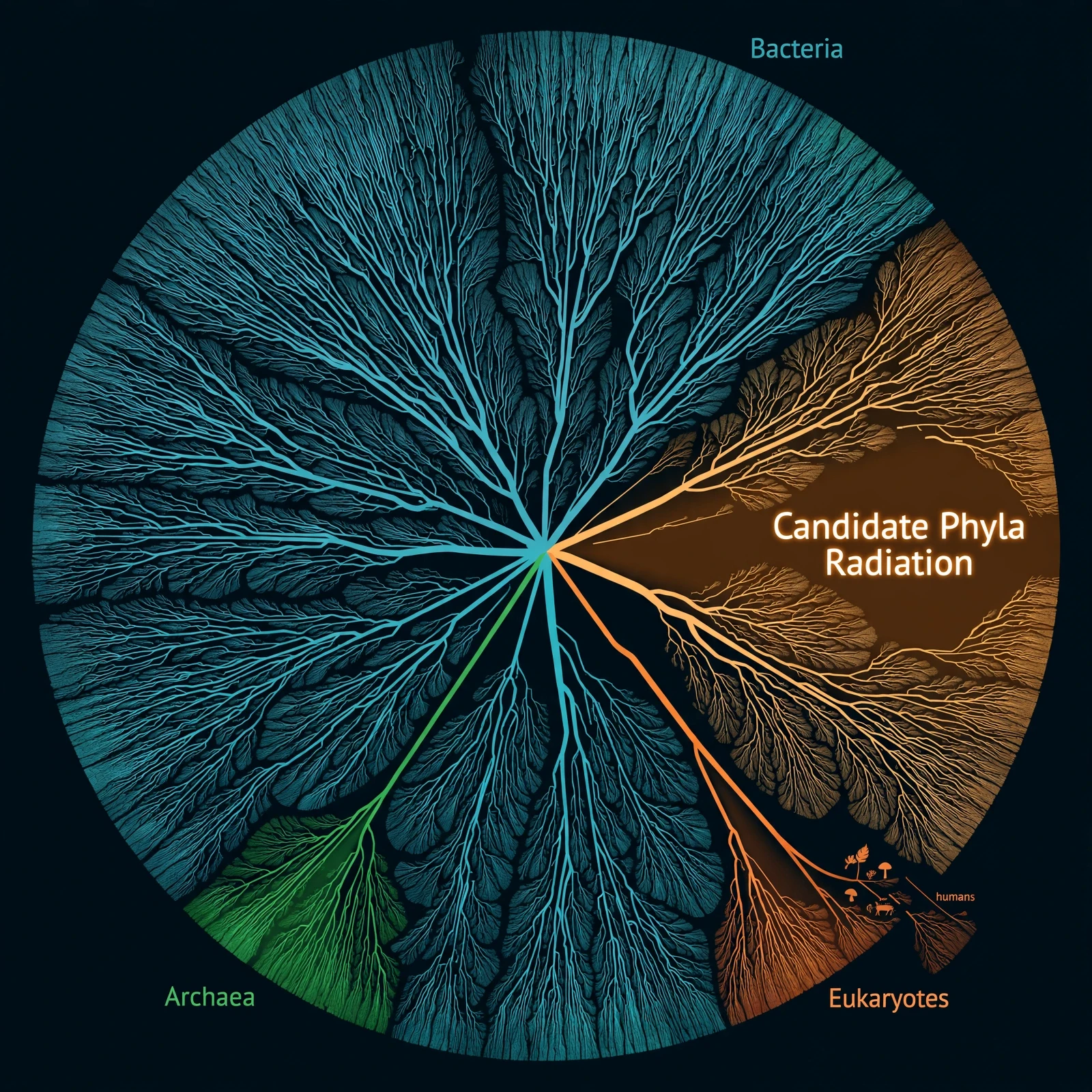
The Hug et al. tree includes 92 named bacterial phyla, 26 archaeal phyla and all five eukaryotic supergroups — and shows that most of life's diversity is bacterial (Hug et al. 2016). Drawn as a circle, with the root at the centre, the bacterial branches fill most of the disc. The eukaryotes occupy a modest wedge. Animals, the group that dominates textbooks and nature documentaries, are a thin sliver inside that wedge. It is a humbling image, and it has become the standard picture of the tree of life for a reason: it is honest about scale.
9.2 The Candidate Phyla Radiation: a large share of bacterial diversity, mostly unknown
The most startling part of the Hug tree is a huge spray of branches labelled the Candidate Phyla Radiation, or CPR. The CPR, highlighted in the Hug tree, is a major radiation of mostly uncultivated bacteria that expanded the known bacterial domain more than five-fold; it contains at least 73 subgroups (The Molecular Ecologist). These are bacteria with tiny genomes and tiny cells, many of them living as symbionts or parasites of other microbes, and almost none of them ever grown in pure culture. Before genome sequencing, they were invisible. On the Hug tree, they occupy a large share of bacterial diversity — the group may comprise more than 15% of the bacterial domain (Brown et al. 2015), and some later estimates put it at around half of all bacterial diversity (Cornish et al. 2022), though the true size of the radiation is still debated.
Think about what that means. A large share of one of life's great domains was unknown to science a decade ago — not unknown in the sense of unclassified, but unknown in the sense of unsuspected. The CPR is a reminder that the tree of life is still being discovered, not merely refined. Every new sampling trip to a deep aquifer or a hydrothermal vent has a real chance of adding branches that nobody predicted.
9.3 GTDB: a genome-based taxonomy that keeps growing
If Hug gave us the picture, the Genome Taxonomy Database — GTDB — gives us the working catalogue. GTDB is a taxonomy built from genomes rather than from shapes or names, and it grows with every new genome sequenced. GTDB Release 10, released in April 2025, spans 732,475 genomes — 715,230 bacterial and 17,245 archaeal — organised into 143,614 species clusters, 136,646 bacterial and 6,968 archaeal (GTDB).
Those numbers are large, and they are also small. GTDB Release 10 represents only 3.3 to 6.5 percent of the conservative global estimate of 2.2 to 4.3 million prokaryotic species — over 95 percent of bacterial and archaeal species remain genomically uncharacterised (Parks et al. 2026). Read that again: after sequencing more than seven hundred thousand genomes, we have genomic data for fewer than one in fifteen of the prokaryotic species thought to exist. The tree of life, for all its new detail, is still mostly blank space. The blank space is not a failure. It is a map of how much exploring remains.
GTDB matters because it gives every genome a place, even when the organism has no proper name, no culture and no photograph. A sequence from a soil sample can be placed on the tree, assigned to a group, and compared with its neighbours — all without anyone ever seeing the cell. That is how the microbial majority is being charted, one genome at a time.
9.4 Open Tree of Life, OneZoom and TimeTree: the tree as a living database
No single paper can hold the whole tree of life. The modern answer is to treat the tree of life as a living database, assembled from thousands of published studies and updated as new ones appear. The Open Tree of Life draft synthesis, published in 2015, combined nearly 500 smaller published trees into a single tree for about 2.3 million named species — the first tree encompassing all of life — yet less than 5 percent of those species had DNA data available (University of Florida). Most branches in that synthesis rested on taxonomy and morphology, not on sequences. That is not a flaw; it is a fair picture of what we knew in 2015. The tree of life was a scaffold, built to be improved.
OneZoom turns that scaffold into something a person can explore. OneZoom maps the connections between 2.2 million living species in a single interactive visualisation, with images of over 85,000 species and extinction-risk colour coding (Imperial College London). You can start at the root, zoom into the mammals, and keep going until you reach a single species of shrew — watching the tree of life unfold like a map. The extinction-risk colours add a second message: the branches you are browsing are not all secure. Some are fading as you look.
TimeTree adds the dimension of time. TimeTree version 5, published in 2022, synthesises divergence times from 4,075 published studies covering 137,306 species; the live site lists 4,185 studies and 150,635 taxon tips (TimeTree). Where the Open Tree says who is related to whom, TimeTree says when they split. Together, the databases turn the tree of life from a figure in a paper into a shared, updatable record — less like a printed map and more like a living atlas.
9.5 The flowering-plant tree: 9,506 species, 1.8 billion letters
The plant tree matters beyond botany. Flowering plants feed us, house us, clothe us and fill our medicine cabinets. Knowing their true relationships helps breeders find wild relatives with useful traits, helps conservationists protect the most distinctive lineages, and helps drug hunters search the right branches for new compounds. The full story of how plant lineages unfolded, from algae to flowers, is told in the companion article on plant evolution. What matters here is the scale of the achievement: nearly ten thousand species, hundreds of genes, more than a billion letters of code — and a tree that, for the first time, lets us see the flowering plants whole.
10. Where the Tree Gets Tangled: The Web of Life
So far this article has told a tidy story: lineages split, branches diverge, and the tree of life grows outward from a single root. That story is largely true — for animals, for plants, for fungi, for most of the twigs we know best. But at the base of the tree of life, among the microbes, the tidy story frays. Genes do not always travel down the branches. Sometimes they jump sideways. Sometimes whole cells move in and never leave. Sometimes two branches fuse back together. The result is a tree with cross-links — a tree that, in places, looks more like a web.
This is not a minor footnote. It is the deepest challenge the tree of life has faced since Darwin drew it, and it deserves a fair hearing. The challenge was raised honestly, answered seriously, and the tree of life survived — changed, but standing. Understanding why is essential to understanding what the tree of life actually is.
10.1 Horizontal gene transfer: genes that jump branches
Horizontal gene transfer, also called lateral gene transfer, is the transfer of genes between unrelated species by mechanisms other than vertical transmission from parent to offspring (LibreTexts). Vertical inheritance is the family route: a parent passes genes to its children. Horizontal transfer is the neighbour route: a microbe picks up a gene from an unrelated microbe living nearby, and passes it on to its own descendants as if it had always owned it.
Microbes do this in three main ways, all of them ordinary parts of microbial life. In transformation, a cell takes up free DNA from its surroundings — the genetic litter left behind by dead neighbours. In transduction, a virus accidentally carries a piece of one host's DNA into the next cell it infects. In conjugation, two cells touch and one passes a loop of DNA directly to the other, like handing over a borrowed book. None of these is exotic. All three happen constantly, in soil, in water, and inside our own bodies.
The consequence for tree building is direct. When Brown and Doolittle reconstructed the tree of life in 1997 using different genes, each gene often produced a fundamentally different tree — a conflict best explained by horizontal gene transfer, especially among prokaryotes (Brown and Doolittle 1997). A gene for one enzyme might say species A is closest to species B. A gene for another enzyme might say A is closest to species C. Both genes are telling the truth — about their own histories. The histories simply differ, because one of the genes jumped branches somewhere along the way.
The practical impact is most visible in medicine. Antibiotic resistance spreads between bacteria largely by horizontal transfer: a resistance gene that evolves in one species can be passed to unrelated species in a hospital ward within days. That is why the companion article on antibiotic resistance treats gene transfer as central, not incidental. A tree that ignored horizontal transfer would miss the very process that makes resistance so hard to contain.
10.2 Endosymbiosis: whole cells that moved in
Horizontal transfer moves genes. Endosymbiosis moves whole cells — and it produced the two most important mergers in the history of the tree of life. More than a billion years ago, an archaeal host cell took in a bacterium that could make energy from oxygen. The bacterium stayed, divided inside its host, and became the mitochondrion — the power plant in nearly every eukaryotic cell. Later, in a separate merger, a eukaryote took in a cyanobacterium that could photosynthesise. That guest became the chloroplast, and its hosts became the algae and plants.
These were not small events. They gave eukaryotes their energy supply and plants their ability to live on sunlight, and they stitched together branches of the tree of life that had been separate for hundreds of millions of years. The genes of the mitochondrion and the chloroplast still carry the signature of their bacterial origins. A tree built from mitochondrial genes tells the history of the mitochondrion, not the history of the animal that carries it. The full story of life's great partnerships, from mitochondria to lichens to the microbes in our guts, is told in the companion article on symbiosis.
Endosymbiosis is a reminder that the tree of life is a tree of cells, not a tree of genes. The host cell and its guest have different ancestors, and both histories are real. A single branching diagram cannot show both at once without cross-links. That is a limitation of the diagram, not a failure of the idea.
10.3 Hybridisation: when branches fuse back together
Branches can also fuse at the species level. Hybridisation happens when two distinct species interbreed and produce offspring that carry genes from both parents. In animals it is relatively uncommon, though famous cases exist — mules, ligers, and the occasional fertile hybrid that founds a new lineage. In plants it is routine: around one in ten plant species is of hybrid origin — a 2017 survey put the average share of presumed hybrid-origin species at close to 11% (2017 survey) — and at least a quarter of plant species hybridize with another species (Mallet 2005; Whitney et al. 2010), sometimes followed by a doubling of the chromosome set that makes the hybrid fertile and reproductively isolated from both parents.
Hybridisation tangles trees in a specific way. A hybrid species has two parents from different branches, so its genes tell two stories. Some genes place it with one parent, others with the other. A tree that forces the hybrid onto a single branch must choose, and either choice hides half the ancestry. The honest drawing is a network, with the hybrid connected to both parents — a small web inside the larger tree.
For most animal groups, hybridisation is a complication at the tips of the tree of life, not a threat to the trunk. It makes the fine branches harder to resolve, but it does not overturn the deeper structure. For plants, where hybridisation is common, tree builders have learned to expect reticulation — net-like patterns — and to report them rather than smoothing them away.
10.4 Doolittle's challenge — and why the tree of life still stands
In 1999, W. Ford Doolittle proposed a phylogenetic model resembling a web or network rather than a tree, hypothesising that eukaryotes evolved from a pool of species sharing genes by horizontal transfer — the "web of life" model (Doolittle 1999). A year later, in Scientific American, he wrote that parts of the tidy scheme scientists had worked out were unravelling — the opening of "Uprooting the Tree of Life" (Scientific American). Doolittle and Bapteste argued in 2007 that the tree's shortcomings require alternative models, while noting the tree remains the most common model in use (Doolittle and Bapteste 2007).
Doolittle's challenge was fair, and it was taken seriously. If genes jump branches freely, what is left of the tree of life? The answer, developed over the following decade, is that the tree of cells survives even when gene trees disagree. Extensive horizontal transfer among prokaryotes means no single gene tree can accurately represent the evolution of entire genomes — yet a tree of cells, of organismal lineages, can still be recovered, which is why the tree concept survives the transfer challenge (Koonin 2009).
The reasoning is straightforward. Genes can jump, but cells divide. A cell lineage — a line of cells descending from a parent cell — has a single history, even if some of its genes arrived sideways. When many genes are analysed together, the shared signal of cell division emerges from the noise of transfer, like a melody emerging from a crowded room. For animals and plants, where horizontal transfer is rare, the tree of life is robust and the cross-links are few. For bacteria and archaea, the tree is real but messier, with a web woven through its lower branches.
That is the modern settlement. The tree of life is not a perfect tree, and it never was. It is a tree with a web at its base, a few fused branches at its tips, and a history of mergers written into its cells. Knowing where it tangles does not weaken it. It tells you exactly where to trust it, and where to look twice.
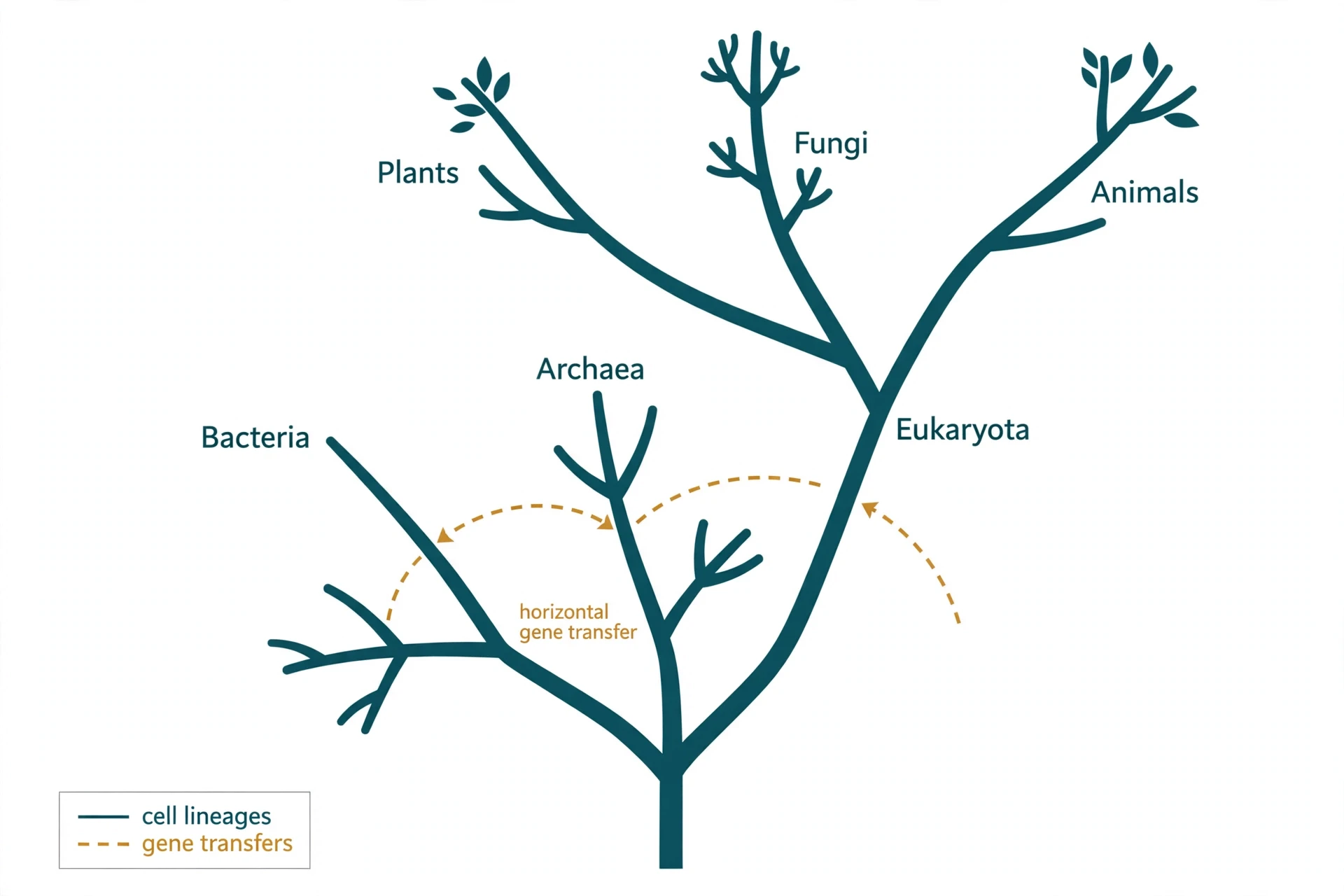
11. The Root and LUCA
Every tree needs a starting point. On an ordinary family tree, the starting point is easy to spot: the oldest ancestor sits at the top, and every branch below leads back to that person. On the tree of life, the starting point is far harder to find. There is no one alive outside the tree of life who can serve as a comparison. Every living thing belongs inside it. So how do scientists decide where the root goes, and what lived there?
The answer takes us back further than any fossil, further than any living species, to a single population of cells that lived about 4.2 billion years ago. Its name is LUCA, the last universal common ancestor. LUCA is one of the most misunderstood ideas in all of biology. It was not the first living thing. It was not the origin of life. It was the last ancestor that every living thing today shares, the furthest point we can reach by tracing backwards from the life around us now.
11.1 How do you root a tree with no outgroup?
In most tree building, rooting is simple. A researcher picks an outgroup, a lineage known to sit outside the group being studied, and the tree is rooted where the outgroup branch joins the rest. The outgroup gives the tree its direction. Time flows away from the root, towards the tips.
That trick fails for the whole tree of life. There is no outgroup to all life, because all life is the group being studied. Nothing alive sits outside it. Scientists therefore need other ways to find the root, and each way leans on a different kind of evidence.
One approach uses ancient gene duplications. Long before LUCA, some genes were copied inside a genome, so a single cell carried two versions of the same gene. Those two copies then evolved separately. By comparing the two copies, researchers can work out which side of the tree split first, because the duplication itself happened before the split. Moody and colleagues used this kind of evidence in their work on the deepest branches of the tree, estimating those branches from ancient vertically evolving genes in a 2022 study in eLife (Moody et al. 2022).
A second approach uses the molecular clock. If a gene changes at a roughly steady rate, the number of differences between two lineages gives a rough measure of the time since they split. Calibrating that clock with microbial fossils and isotope records lets researchers place dates on the deepest splits, even when no fossil of the organism itself survives. That is the method behind the modern date for LUCA, as we will see in the next sections.
None of these methods gives a root carved in stone. They give a best-supported placement, one that can shift as new genomes arrive. That is how science is supposed to work. The root is a hypothesis, tested against every new piece of evidence.
11.2 LUCA: not the first life, the last shared ancestor
The name says it plainly, once you slow down and read it. LUCA is the last universal common ancestor. Last, not first. Every living thing today descends from LUCA, but LUCA itself descended from earlier life. It had ancestors, cousins, and neighbours, and all of those other lineages are now extinct.
Quanta Magazine put it in a single clear sentence in 2024: LUCA is the furthest point in evolutionary history reachable by working backwards from what is alive today, and it is not the origin of life and not the first cell (Quanta Magazine). That distinction matters. The origin of life is a separate question, about how chemistry first became biology. LUCA is a later question, about the ancestor of everything that survived.
LUCA is the same idea, stretched across all of life. It is the ancestor at the reunion of every bacterium, archaeon, fungus, plant, and animal alive today. The life that came before LUCA left no direct descendants. We know it must have existed, because LUCA was already a complex cell, far too complex to have been the first attempt at life. But its predecessors are gone, and their genes survive only in the traces they left in LUCA's own genome.
That is why the origin of life and LUCA belong in different conversations.
11.3 What LUCA was like — the 2024 portrait
For a long time, LUCA was little more than a dot at the base of the tree of life, a placeholder with no face. That changed in 2024, when a team led by Edmund Moody published a detailed reconstruction in Nature Ecology and Evolution. By comparing the genes shared across Bacteria and Archaea, and by dating the splits with gene duplications calibrated against microbial fossils and isotope records, the team built the clearest portrait of LUCA yet (Moody et al. 2024).
The headline date is striking. LUCA lived about 4.2 billion years ago, with a range of 4.09 to 4.33 billion years. Earth itself formed about 4.5 billion years ago, so LUCA lived only about 400 million years after the planet formed, in a period long thought too harsh for life. That short gap is one of the most surprising findings of the study. Life did not take its time getting started and then slowly build up to LUCA. By the time LUCA lived, life was already well established.
LUCA was not a bare scrap of chemistry. Its genome was at least 2.5 million bases long, in a range of 2.49 to 2.99 million bases, encoding around 2,600 proteins. That is comparable to a modern prokaryote. It was a prokaryote-grade cell, with no nucleus, living without oxygen as an anaerobic acetogen, a microbe that makes its living from hydrogen and carbon dioxide. And it already possessed an early immune system, which tells us something remarkable: even 4.2 billion years ago, there were viruses or other genetic parasites to defend against. LUCA was not living alone in a quiet world. It was part of an ecosystem, with predators and competitors of its own.
The portrait also tells us that LUCA was one of many. If LUCA already had an immune system, a large genome, and a working metabolism, then other lineages must have been alive at the same time, sharing genes, competing for resources, and in some cases preying on each other. LUCA is the one whose descendants survived. The rest are gone, leaving no living trace except the genes they may have passed to LUCA's line before they vanished.
Here is LUCA at a glance, with the numbers from the 2024 study.
Feature | What the 2024 study found |
|---|---|
Age | About 4.2 billion years ago (range 4.09–4.33 billion years) |
Genome size | At least 2.5 million bases (range 2.49–2.99 million bases) |
Proteins encoded | About 2,600 proteins, comparable to a modern prokaryote |
Cell type | Prokaryote-grade cell, with no nucleus |
Metabolism | Anaerobic acetogen, living without oxygen |
Defences | An early immune system, showing it faced viruses or other parasites |
What it was not | Not the origin of life, and not the first cell |
What it was | The last ancestor shared by all life alive today |
Table 4: LUCA at a glance. All figures from Moody et al. 2024, Nature Ecology and Evolution.
11.4 What the root tells us, and what it cannot
The root of the tree of life tells us where to start reading. On the best-supported placement, Bacteria split from the line leading to Archaea and eukaryotes very early — though the exact position of the root is still debated — and it tells us that the ancestor of all surviving life was already a capable, complex prokaryote. It sets the direction of time for every branch above it.
What it cannot tell us is what came before LUCA. The root is a horizon, not a window. Beyond LUCA, the branches that might have shown us the first cells are gone. We can infer that earlier life existed, because LUCA was too complex to be first, but we cannot draw its tree.
12. Deep Branches in Focus
If LUCA is the root, the deep branches are the first great forks above it. They are also the hardest branches to resolve. The splits happened billions of years ago. Most of the lineages that were alive at the time are extinct. The survivors have had billions of years to change, lose genes, and swap genes with their neighbours. The result is a set of questions that have stayed open for years, even as genomes have piled up by the hundred thousand.
This section looks at three of those questions: where eukaryotes came from, which animal group branched off first, and where the great eukaryotic groups sit. None of them has a settled answer yet. That is the point. The tree of life is not a finished diagram. At its deepest levels, it is still being drawn.
12.1 Eukaryote origins: Asgard archaea and eukaryogenesis
For most of the twentieth century, eukaryotes looked like a separate creation. Our cells have a nucleus, a complex internal skeleton, and compartments that sort and move cargo around. Bacteria and archaea have none of that, or so it seemed. Then, in 2015, genomes recovered from sediments near Loki's Castle, a hydrothermal vent system in the North Atlantic, revealed a new archaeal group called Lokiarchaeota, and with it a new idea: eukaryotes branch from within Archaea (PNAS 2026).
Lokiarchaeota was the first member of what became the Asgard group, named after the home of the Norse gods. The group now includes Loki-, Thor-, Odin- and Heimdallarchaeota. Asgard archaea carry many genes previously thought exclusive to eukaryotes, involved in trafficking, the ubiquitin system, endosomal sorting, and cytoskeleton formation. In plain language, these archaea already owned some of the molecular toolkit that eukaryotes later used to build complex cells. The boundary between archaeon and eukaryote began to look less like a wall and more like a slope.
The story took a vivid turn in 2020, when researchers reported the first cultivated Asgard archaeon, Candidatus Prometheoarchaeum syntrophicum, strain MK-D1. This microbe has long branching protrusions and degrades amino acids syntrophically with partner microbes, living in close partnership with other cells that consume its waste products (Zhang et al. 2025). It looks, in shape and lifestyle, like a cell that could have hosted a partner inside itself. That is the kind of partnership eukaryogenesis required: one cell taking another cell inside, and keeping it.
The largest step forward came in 2025. Zhang and colleagues published a study in Nature, "Deep origin of eukaryotes outside Heimdallarchaeia within Asgardarchaeota", built from 223 new near-complete Asgard genomes. The team identified 16 new lineages at genus level or higher, and inferred that eukaryotes evolved before the diversification of all sampled Heimdallarchaeia, supporting the hydrogen hypothesis of eukaryogenesis (Zhang et al. 2025). The hydrogen hypothesis holds that the first eukaryote arose from a partnership in which one partner produced hydrogen and the other consumed it, a metabolic handshake that became a merger.
The same study placed the last Asgard-eukaryote common ancestor before the Great Oxidation Event, the period when oxygen first built up in the atmosphere. That ancestor was probably an anaerobic hydrogen-dependent acetogen, a microbe living without oxygen and making its living from hydrogen. Our deepest ancestor, in other words, was a microbe that would have found oxygen poisonous.
What does this mean for the tree of life? It means the three-domain picture from §5 needs a footnote. If eukaryotes sit inside Archaea, then Archaea as traditionally drawn is not a clean, separate domain. The tree of life still has three great trunks in one sense, but the eukaryote trunk grows out of the archaeal one. That is why some researchers now speak of a two-domain tree, with Bacteria on one side and Archaea plus eukaryotes on the other. The change is not a rejection of the earlier work. It is what happens when new genomes sharpen an old picture. One disagreement is still open: the 2026 PNAS review places eukaryotes within Heimdallarchaeia, with Hodarchaeales as a leading candidate for the closest archaeal relative — while the 2025 Zhang study places them outside Heimdallarchaeia — so the outside-versus-inside question is itself an active disagreement between the two studies, not a settled result.
12.2 The animal root: sponges vs ctenophores
Turn from microbes to animals, and the deepest question is simpler to state and just as hard to settle: which animal group branched off first? For more than a century, the answer seemed obvious. Sponges are the simplest animals. They have no nerves, no muscles, no gut, and no true tissues. They filter water through a body that is barely more organised than a colony of cells. Surely, the reasoning went, sponges must be the sister group to all other animals, the first branch off the animal trunk.
Then, in 2008, a phylogenomic study by Dunn and colleagues proposed the opposite. Based on data from 29 species representing 21 animal phyla, the team argued that ctenophores, the comb jellies, not sponges, are sister to all other animals (Dunn et al. 2008). Comb jellies are graceful, transparent swimmers with rows of beating combs, a nervous system, and muscles. If they branched first, then the simple sponge body plan is not the starting point of animal evolution. It is a later simplification, or a separate path entirely.
That claim set off one of the longest arguments in modern phylogenetics. Other datasets, built from different genes and different methods, kept pointing back to sponges first (Simion et al. 2017). The two answers traded places as methods improved and sampling grew. Neither side could land a clean win, because the split happened in a rapid radiation that left short internal branches and weak signals.
A new kind of evidence arrived in 2023. Schultz and colleagues used chromosome-scale synteny, the order of genes along chromosomes, from new ctenophore and sponge genomes. They found rare, irreversible chromosome fusion-and-mixing events uniting sponges with bilaterians, cnidarians, and placozoans to the exclusion of ctenophores, a pattern that supports ctenophores as sister to other animals (Schultz et al. 2023). Chromosome rearrangements of this kind are rare and hard to reverse, so sharing one is strong evidence of shared ancestry. On that character set, the support was very high.
Even so, the debate remains unresolved. A 2026 synthesis preprint, not yet peer-reviewed, notes that traditional datasets tend to support the sponge-first hypothesis while high-resolution data increasingly favour ctenophore-first (Preprints.org 2026). That split is the honest state of the field. Different kinds of data point in different directions, and no single study has reconciled them.
So this article declares no winner. If you read a textbook that states sponge-first as settled fact, it is out of date. If you read a news story that states ctenophore-first as settled fact, it is overstating the case. The animal root is genuinely open, and the reason it matters is not trivia. Which group branched first shapes how we read the origin of nerves, muscles, and the gut. If sponges branched first, those features evolved once, after sponges split off. If ctenophores branched first, the story is more tangled: either those features evolved twice, or sponges lost them. The root decides which story we tell about our own deep history, and the evidence has not yet decided.
12.3 Where plants, animals and fungi sit
Animals are one branch of the eukaryotes, and plants are another, and the flowering-plant branch has been mapped in remarkable detail. The 2024 flowering-plant tree from Zuntini's team — 9,506 species, 7,923 genera, every order and family, drawn from 353 nuclear genes and 1.8 billion letters of code — is the largest of its kind yet (Zuntini et al. 2024). That tree shows what a well-sampled eukaryote branch looks like: thousands of species, dense sampling, and strong support for most splits. Animals, by contrast, radiated in the Cambrian explosion, in a burst that left short branches and faint signals.
Plants and animals also illustrate how the tree of life records great mergers, not just splits. The chloroplasts inside plant cells were once free-living bacteria, taken inside an early eukaryote and kept. The mitochondria inside animal cells, and plant cells too, were once free-living bacteria as well. Those events are covered in more detail in the symbiosis article, but they belong here too, because they show that the deep branches of the tree of life were shaped by cells joining together, not only by cells splitting apart.
12.4 Why deep branches are the hardest to resolve
Three forces make deep branches hard, and they all grow stronger with age. The first is time itself. A split that happened a billion years ago has had a billion years of later changes piled on top of it. Genes mutate, lineages lose genes, and the original signal fades under the noise. The deeper the node, the fainter the signal.
The second is extinction. About 99 percent of all species that ever lived are thought to have gone extinct, so any tree of living species is a minuscule subset of the full tree of life, with most branches missing (Georgia Tech Bio 1220). Extinct lineages are the missing witnesses. When they vanish, they take with them the intermediate forms that would have shown how one branch led to another. Deep nodes lose their stepping stones first, because the most time has passed for those stones to disappear.
The third is gene conflict. Brown and Doolittle's 1997 experiment — rebuilding the tree from different genes and watching the results disagree — pointed to horizontal transfer among prokaryotes as the cause (Brown and Doolittle 1997). At deep levels, that conflict is not a rare exception. It is common. Different genes have different histories, and the species tree is the pattern that emerges when many genes are weighed together, not the story of any single gene.
Where exactly do eukaryotes sit inside Asgard? Zhang's 2025 study puts them outside Heimdallarchaeia, the 2026 PNAS review puts them inside it, with Hodarchaeales the leading candidate for closest archaeal relative — so whether eukaryotes sit outside or inside remains actively disputed, and the precise Asgard lineage that is our closest archaeal relative is still being narrowed down as new genomes arrive.
Which animal group branched first, sponges or ctenophores? Traditional datasets lean sponge-first, high-resolution data lean ctenophore-first, and the question remains unresolved.
Where is the root of the eukaryotes themselves? The first split among living eukaryotes, and how the great eukaryotic groups relate to each other, is still being refined, because the early eukaryotic radiation was rapid and much of its diversity is microbial and poorly sampled.
13. The Human Branch
Somewhere near the tips of the tree of life, on a small twig that is easy to miss if you are looking at the whole diagram, sits a primate that learned to read trees. That primate is us. The human branch is not the top of the tree of life. It is not the goal of the tree of life, and it is not the longest branch. It is one twig among millions, and its story is best told by placing it carefully among its neighbours.
13.1 Where humans sit: one twig among primates
Humans are apes. That sentence still surprises people, but on the tree of life it is plain. We sit inside the apes, inside the primates, inside the mammals, inside the vertebrates, inside the animals. Each of those groups is a clade — an ancestor with all of its descendants — and we belong to every one of them. There is no separate human branch standing apart from the apes. There is only the ape branch, with humans as one of its tips.
That placement carries a simple lesson. We are not outside nature, looking in. We are one lineage inside it, shaped by the same processes that shaped every other lineage on the tree of life: mutation, drift, selection, and split after split after split.
13.2 The primate tree and the ape splits
The primate tree is a good tree to learn on, because it is well sampled and well dated. Its tips include lemurs, monkeys, and apes, and its nodes mark the splits that produced them. The ape splits are the ones that matter most for our own story: the split that separated orangutans from the line leading to gorillas, chimpanzees, and humans; the split that separated gorillas; and the split that separated the human line from the chimpanzee and bonobo line.
That last split is the one people ask about most, and it is the one where two numbers circulate. The commonly quoted figure is about six million years ago. The authoritative range, from the sibling article on the molecular clock, is 4.7 to 8.7 million years (Molecular Clock). This article uses that range as the authoritative figure, so the two live articles agree. About six million years is the commonly quoted midpoint, a handy shorthand, not a separate measurement. The range is the honest statement: the split happened somewhere in that window, and different genes and different calibrations place it at different points inside it. The earlier ape splits are older: the gorilla line split from the line leading to humans and chimpanzees roughly 7–10 million years ago, and the orangutan line split earlier still, roughly 12–15 million years ago — approximate figures, since different genes and calibrations give somewhat different dates (Glazko and Nei 2003).
The ancestor at that node was neither a human nor a chimpanzee. It was an ape that lived several million years ago, and its descendants split into two lines. One line led, through many further splits and extinctions, to modern humans. The other led, through its own splits, to modern chimpanzees and bonobos. Both lines have been evolving for exactly the same length of time since that split. Neither is a living fossil. Neither stopped evolving.
I first felt the weight of that idea not in a lecture hall but in a zoo, standing in front of a chimpanzee enclosure and watching a young chimp solve a puzzle with a stick. The keeper beside me said, quietly, that the animal was not a failed human or a primitive version of us, but a cousin who had taken a different road from the same starting point. I have carried that sentence with me ever since, because it captures in plain language what the tree of life says in branches and nodes: we share an ancestor, not a ladder.
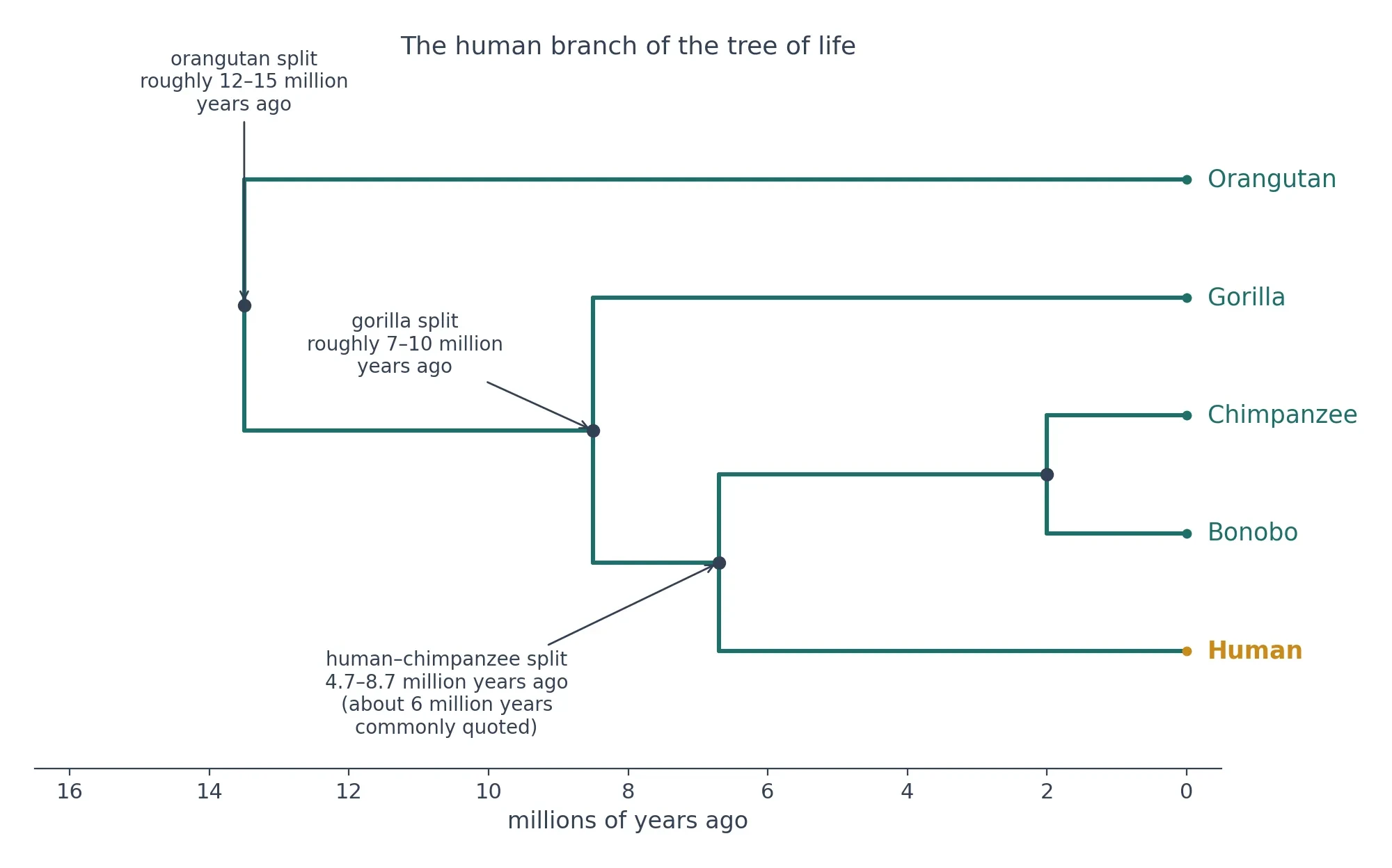
13.3 How genomes revised the human tree
Before genomes, the human tree was drawn mostly from bones and teeth. Fossils could show that a skull was more human-like or more ape-like, but they could not measure how much DNA two living species share. Genomes changed that, and the numbers they returned were startling in both directions: strikingly similar, and strikingly different.
Humans and chimpanzees share about 98.8 percent of their DNA in alignable protein-coding sequence. The 1.2 percent difference amounts to around 35 million single-letter discrepancies across a roughly 3-billion-base-pair genome (IFLScience). That is the paradox of the human branch in a single pair of numbers. We are almost identical to chimpanzees in the parts of the genome that can be lined up and compared, and yet 35 million differences is a large number of differences. Small percentages, spread across a large genome, add up to a large absolute count, and a small number of those differences have large effects.
One much-discussed example is FOXP2, a gene involved in speech and language. The human FOXP2 gene differs from the chimpanzee version by 5 nucleotides, 2 of which change amino acids (Biology LibreTexts). Five letters out of a whole genome sounds like nothing. Two amino acid changes sound like even less. Yet those changes sit in a gene that helps wire the brain for the fine motor control that speech requires, and they are part of the reason a five-letter difference is worth studying at all. The lesson is not that FOXP2 alone made us human. No single gene did that. The lesson is that the tree of life is built from differences that are small in count and large in consequence.
Genomes also revised the human tree in a more structural way. Humans have 23 pairs of chromosomes. Chimpanzees have 24 pairs. The human chromosome 2 is a fusion of two ancestral ape chromosomes (KnowAnimals). Two chromosomes that remain separate in chimpanzees joined end to end in the human line. The fusion left a visible signature in the DNA, a second centromere and telomere sequences in the middle of the chromosome where the two ends met. It is a physical record of a split, written into the genome itself.
For the wider story of how our species evolved, and for the fossil evidence behind the hominin branch, see the human evolution article. For the genome in full, including the comparison with chimpanzees in its wider context, see the human genome article. The dating method behind the split dates in this section is the molecular clock, explained in the molecular clock article.
13.4 What the human branch does — and does not — mean
The human branch means that we are primates, that we are apes, and that our closest living relatives are chimpanzees and bonobos. It means our lineage split from theirs 4.7 to 8.7 million years ago, and that both lineages have been evolving ever since. It means we share most of our protein-coding DNA with chimpanzees, and that the differences, though small in percentage terms, number in the tens of millions.
It does not mean that humans are more evolved than chimpanzees. There is no such measurement on the tree of life. Every living tip has had the same total time to change since the root. A chimpanzee is not a human that stopped halfway. A human is not a chimpanzee that went further. Both are present-day endpoints of their own branches, shaped by their own histories.
It does not mean that humans evolved from chimpanzees. That is the most common misunderstanding in this whole area, and the tree of life answers it directly. Humans and chimpanzees share a common ancestor that was neither. Chimpanzees have been evolving for just as long as humans since that split (IFLScience). To say we evolved from chimpanzees is to mistake a cousin for a parent, and to mistake a living tip for a node.
One more wrinkle complicates even this tidy branch: admixture. Modern humans interbred with Neanderthals after leaving Africa, so most people with ancestry outside Africa carry roughly 1–2% Neanderthal DNA (Green et al. 2010), and people of Melanesian ancestry carry roughly 4–6% Denisovan DNA. On a strict tree, that gene flow is a cross-link, not a split — a reminder that even the human branch carries a little web in it.
14. What Trees Are Used For
A tree of life is not only a picture for textbooks. It is a working tool, used every day in conservation, in medicine, in forensics, and in the search for new drugs. The uses below are concrete, and each one leans on the same idea: relatedness predicts similarity. Close relatives tend to share traits, genes, and vulnerabilities. A tree of life tells you who the close relatives are, and that knowledge tells you where to look, what to protect, and what to expect next.
14.1 Classification: naming the branches
The first use of a tree is the oldest one: classification. Naming and grouping organisms is a separate job from drawing their history, but the two jobs inform each other. A good classification groups organisms by their shared ancestry, so that a name tells you something about relationships, not just about appearance. That is the complement to the animal classification article, which covers taxonomy in its own right. This article covers the tree of life that classification should reflect.
The rule is simple to state and hard to follow in practice: on the tree of life, a named group should be a clade — one ancestor with all of its descendants included. When a group leaves out some descendants, or lumps together lineages from different branches, the name misleads. The classic example is the old grouping of reptiles, which left out birds even though birds descend from inside the reptile branch. A tree exposes that mistake at a glance, because the bird tip sits inside the reptile clade. Classification that follows the tree of life avoids it.
Trees of life also guide what to name next. When a new species is described, its place on the tree decides its genus, its family, and its wider group. When a tree shows that a genus is split across two branches, taxonomists know the genus needs revising. The tree of life is the test that a classification must pass.
14.2 Conservation: EDGE species and phylogenetic diversity
The most direct conservation use of the tree of life is the EDGE of Existence programme, run by the Zoological Society of London since 2007. EDGE scores species by two things: Evolutionary Distinctiveness, measured from a phylogeny, and Global Endangerment, taken from the IUCN Red List (ZSL EDGE of Existence). An EDGE species is a threatened species with few or no close relatives. Lose it, and you lose a long, lonely branch of the tree of life, with no close cousin to carry its history forward.
The distinctiveness rankings make the idea vivid. The most evolutionarily distinct mammal in the world is the aardvark. The most distinct amphibian is the Mexican burrowing toad. The most distinct bird is the oilbird. The most distinct reptile is the tuatara (ZSL EDGE of Existence). None of these animals is famous in the way a tiger or a panda is famous. Each of them sits at the end of a long branch with few neighbours, and each of them carries a large share of unique evolutionary history in a single species.
The scale of the programme is large. There are over 550 EDGE mammal species, about 10 percent of all mammals, and over 900 EDGE amphibian species, about 13 percent of all amphibians (ZSL EDGE of Existence). Those numbers show that distinctiveness is not rare. A tenth of all mammals are both threatened and evolutionarily distinct. Conservation that ignores the tree would miss them.
The programme has also moved from species to places. EDGE Zones, identified in 2024, make up 0.7 percent of Earth's surface but are home to one-third of the world's four-legged EDGE species (EDGE of Existence programme). Protecting a small area can therefore protect a large share of distinct evolutionary history, if the area is chosen with the tree in mind. That is a practical result: a map drawn from a phylogeny tells conservationists where a limited budget will save the most history.
The metric itself has been updated. The EDGE2 protocol, published by Gumbs and colleagues in 2023, updated the metric to account for the extinction risk of close relatives and to express scores as the amount of phylogenetic diversity expected to be lost, in millions of years, that conservation could avert (Gumbs et al. 2023). Phylogenetic diversity sums the lengths of phylogenetic branches to quantify the unique and shared evolutionary history of a set of species, and it is the basis for prioritising places as well as species (Nature Communications 2024). In plain terms, EDGE2 asks not only how distinct a species is, but how much history would vanish with it, and how much of that loss conservation could prevent.
14.3 Epidemiology: reading viral trees in real time
Viruses evolve fast, and the viral branches of the tree of life can be read in real time. When a new viral genome is sequenced, researchers place it on a tree with other genomes from the same outbreak or the same season. Its position shows which other samples it is most closely related to, and how recently they shared an ancestor. That placement is the starting point for tracing how a virus spreads, which variants are growing, and where a new variant came from.
The logic is the same as in the rest of this article. Relatedness is decided by the most recent shared node, not by appearance or by geography. Two viral samples from the same city can sit far apart on the tree, if they came from separate introductions. Two samples from different continents can sit close together, if they share a recent ancestor. The tree corrects the guess that nearness in space means nearness in ancestry.
Viral trees also show change over time. A phylogram, with branch lengths proportional to change, reveals which lineages are accumulating mutations quickly and which are stable. A tree built from many genomes can show a new variant branching off and growing, while older variants fade. That is why public health teams build viral trees during outbreaks: the tree turns a pile of sequences into a picture of spread that can help inform testing, travel advice, and vaccine updates — the approach used by platforms such as Nextstrain, which tracks SARS-CoV-2 evolution in real time (Nextstrain). For the wider story of how viruses evolve, see the virus evolution article.
14.4 Forensics, food and drug discovery
The same logic of the tree of life reaches into forensics and food safety. When the source of an outbreak or a case of food poisoning needs identifying, researchers sequence the microbes involved and place them on a tree. Whole-genome sequencing is now the standard tool public-health agencies use to link cases of food poisoning to the same source of contamination (PNAS 2024). The samples that cluster tightly together share a recent ancestor, and that clustering can point to a common source. A tree does not replace laboratory testing or field investigation, but it narrows the search. It tells investigators which samples belong together and which do not, and that distinction can separate a single contaminated batch from unrelated cases that happen to look similar.
Wildlife forensics works the same way. A seized sample of ivory, timber, or meat can be sequenced and placed on a tree of known species and populations. Its position shows which species it came from, and sometimes which population within that species. That placement can be evidence in court — in one Kenyan ivory-trafficking conviction, genetic tests tying tusks from different shipments to a single cartel were described as directly usable for courtroom prosecution (Yale Environment 360) — because it rests on the same relatedness logic as every other tree in this article: the closest relatives on the tree are the closest relatives in reality.
Drug discovery uses the tree of life in the opposite direction, from the known to the unknown. Zuntini's 2024 flowering-plant tree spans 9,506 species in 7,923 genera, with all 64 orders and 416 families represented, built from 353 nuclear genes (Zuntini et al. 2024). A tree of that breadth lets researchers ask a practical question: if one plant in a group makes a useful compound, are its close relatives likely to make similar compounds? Often the answer is yes, because related plants share the biochemical pathways that make those compounds — biologists hunting for a cheaper source of the cancer drug taxol, first found in the Pacific yew, found a related compound in the leaves of its close relative the European yew (UC Berkeley, Understanding Evolution). The tree becomes a map for searching, pointing researchers towards the relatives most likely to hold something useful, instead of testing species at random.
Interactions between species add another layer. When two lineages evolve together, in a long-running partnership or arms race, their trees can mirror each other. That is the subject of the coevolution article, and it matters for drug discovery and for agriculture, because a tree that shows how a pest and its host have tracked each other can predict how the pest will respond to a new control. In each of these uses, the tree is doing the same job: turning relatedness into a prediction, and turning a prediction into a decision.
15. Common Mistakes Reading Trees
Trees of life are easy to misread, and the mistakes are predictable. They follow from habits we bring from other diagrams: reading left to right, reading top to bottom, and assuming that what is drawn near must be related. A phylogenetic tree follows different rules, and this section states them plainly. Keep the checklist at the end. It is short, and it catches most errors before they happen.
15.1 Ladder thinking: evolution as a staircase
The first mistake is to read a tree as a ladder, with simple organisms at the bottom and complex ones at the top, and humans on the highest rung. The tree of life is not a staircase. It is a branching bush, with many tips alive at the same time. No tip is higher than another in any biological sense. The vertical position of a tip is a drawing choice, not a rank.
Ladder thinking has a long history, going back to trees that placed humans at the top as a matter of design rather than evidence. Modern trees do not do that. They place tips where the branching pattern puts them, and they rotate branches freely, because rotation changes nothing about relationships. A human tip drawn at the top of a page is no more evolved than a sponge tip drawn at the bottom. Both have had the same span of time to change since the root.
15.2 "More evolved" and the leftmost-tip trap
The second mistake is the phrase "more evolved". It sounds like a measurement, but it is not one. Every living species has been evolving for exactly as long as every other living species, since the root of the tree of life. A lineage that branches early has still been evolving for the same total time as a lineage that branches late. A living species is never the ancestor of another living species, and an early-branching lineage is not a living fossil that stopped changing (Georgia Tech Bio 1220).
The leftmost-tip trap is the visual version of the same error. On a tree drawn left to right, the leftmost tip looks oldest or most primitive. It is neither. Swapping the labels of two sister taxa gives a topologically equivalent tree, and the leftmost tip is neither the oldest nor the most primitive (Georgia Tech Bio 1220). Tip order is arbitrary. The tree's meaning lives in its nodes, not in the order of its tips along the page.
15.3 Reading across the tips instead of back to the nodes
The third mistake is to judge relatedness by looking across the tips, as if the species drawn next to each other must be close relatives. They need not be. In a five-species tree, the closest relative of species C is not necessarily the species drawn next to it. Relatedness is decided by the most recent shared node, not by left-to-right order (Georgia Tech Bio 1220).
The correction is a single rule, and it replaces most tree-reading confusion: what matters is how species connect through nodes as you move away from the root — nothing else about the drawing does (University of Minnesota phylogenetics guide). To find the closest relative of any species, trace its branch back to the first node, and see which other branch shares that node. That is the answer. Tip distance, tip order, and visual nearness are all irrelevant.
15.4 Similarity is not relatedness
The fourth mistake is to assume that species that look alike must be closely related. Often they are, but not always. Similar environments can shape unrelated lineages in similar ways, a process called convergent evolution. Sharks and dolphins look alike because both live fast lives in open water, not because they share a recent ancestor. One is a fish, the other a mammal, and their shared node lies far back on the tree.
The tree of life is the tool that catches this error. Two species can look similar and sit far apart, or look different and sit close together. Humans and chimpanzees look different in obvious ways, yet they share a recent ancestor. A bat and a bird both fly, yet their flying evolved separately. Appearance is evidence, but it is only one kind of evidence, and the tree weighs it against genes, fossils, and anatomy together. When appearance and the tree disagree, trust the tree, and ask what shaped the appearance.
15.5 Assuming the tree is finished
The fifth mistake is to assume the tree is finished, that scientists know all the branches and only need to fill in a few details. The tree of life is far from finished. The first synthesis covering all named life held roughly 2.3 million species, and DNA data backed fewer than one in twenty of them — most branches still rest on taxonomy and anatomy rather than sequences (University of Florida 2015). The Open Tree authors themselves stress the tree is far from perfect, with many organisms whose relationships are not well understood scientifically.
A tree of life is a hypothesis you can test, not a family portrait. Which branching pattern it prefers can shift as sampling, data or methods improve (How to Read an Evolutionary Tree 2025). That is not a weakness. It is what makes a tree scientific. A diagram that cannot change when new evidence arrives is not a hypothesis. It is a poster. The tree of life changes because the evidence keeps growing, and it will keep changing for as long as new species are described and new genomes are sequenced.
Keep this checklist. It fits on a card, and it catches the five mistakes above before they take hold.
Ladder thinking: a tree is a branching bush, not a staircase. No tip is higher than another.
"More evolved": every living lineage has had the same span of time to change. No living species is the ancestor of another.
Reading across the tips: relatedness is decided by the most recent shared node, never by tip order or tip distance.
Similarity is not relatedness: look-alike species can sit far apart. Check the nodes, not the appearance.
Assuming the tree is finished: the tree is a testable hypothesis. It changes as new evidence arrives, and that is a strength.
16. Myths and Misconceptions
A diagram as famous as the tree of life collects misunderstandings the way a magnet collects pins. Most of them sound reasonable. Most of them fall apart the moment you trace a real branch back to its node. Here are the eight I hear most often, stated plainly, then corrected with what the evidence actually shows.
1. "Humans evolved from chimpanzees." No. That is wrong, and it is wrong in a way that matters, because it gets the shape of the tree of life backwards. Humans did not evolve from chimpanzees, and chimpanzees did not evolve from humans. The two lineages split from a shared ancestor about six million years ago — the commonly quoted midpoint of the 4.7 to 8.7 million year range given in our companion guide to the molecular clock — and that ancestor was neither a human nor a chimpanzee. Since the split, chimpanzees have been evolving for just as long as we have. They are not frozen versions of our past. They are our cousins, with their own long history of change. The shared DNA tells the same story: about 98.8 percent of the two genomes matches in alignable protein-coding sequence, while the 1.2 percent difference adds up to around 35 million single-letter discrepancies across a roughly three-billion-base-pair genome. A close cousin is not a parent. Once you see the split as a fork, the myth has nowhere left to stand.
2. "The tree of life is finished. Scientists know all the branches." Far from it. The first tree spanning all of life, the Open Tree of Life's 2015 synthesis, wove together almost 500 published trees to cover some 2.3 million named species — yet DNA data existed for under five percent of them. The microbial picture is thinner still. GTDB Release 10, from April 2025, holds 732,475 genomes in 143,614 species clusters — yet that covers just 3.3 to 6.5 percent of the 2.2 to 4.3 million prokaryotic species in the conservative global estimate, leaving over 95 percent of bacterial and archaeal species genomically uncharacterised. A tree with most of its twigs still missing is a work in progress, not a finished map.
3. "Evolution always makes things more complex." The tree of life shows no single direction toward complexity. Complexity was already present at the very base of the tree we can reconstruct. LUCA, the last universal common ancestor, had a genome of at least 2.5 million base pairs encoding around 2,600 proteins, comparable to a modern prokaryote, and already possessed an early immune system. Bacteria, meanwhile, hold most of life's diversity. Hug's 2016 tree counts 92 named bacterial phyla and 26 archaeal ones beside all five eukaryotic supergroups — and shows most of life's diversity is bacterial. If evolution always built upward toward complexity, the tree of life would look like a staircase with bacteria at the bottom and humans at the top. It looks nothing like that. It looks like a vast bush of microbes, with animals and plants as late, small offshoots. Some lineages gain elaborate structures. Others stay small and simple for billions of years and thrive. The tree records both without ranking them.
4. "If two species look alike, they must be closely related." Likeness can lie. Homologous characters come from shared ancestry and tell us about relationships, while analogous ones merely resemble each other through convergent evolution and mislead trees when mistaken for homology. That is why tree builders do not group species by a general impression of similarity. They group them by shared derived characters, called synapomorphies, which are the only characters that can establish relationships. Shared ancestral characters are too widespread, and unique traits are too restricted, to tell us about relationships within a group. On the tree of life, the test is always descent, never resemblance alone.
5. "Bacteria are primitive and simple." Bacteria are not simple or primitive. The Hug tree shows bacterial diversity dwarfs that of eukaryotes, and most of life's genetic diversity is microbial. The Candidate Phyla Radiation alone — a major radiation of mostly uncultivated bacteria, highlighted in the Hug tree — enlarged the known bacterial domain more than five-fold and holds at least 73 subgroups. A group that has been evolving for more than three billion years, colonising boiling springs, deep rock, frozen soil and the inside of your gut, is not a rough draft of life. It is life's main event.
6. "A species on a side branch is a failed experiment, an evolutionary dead end." A side branch is simply a branch. On a tree, all living lineages are the same age in the only sense that matters — each has been changing since the root, however early it branched off. No living species is the ancestor of another living species, so there is no main line to fall off. A tuatara or an aardvark is not a leftover that evolution forgot. It is a survivor whose lineage found a way of life that kept working while countless other branches vanished. Extinction has pruned the tree relentlessly — as §12.4 explains, almost everything that ever lived is gone, and the living tree is only the surviving remnant. Against that background, still being here is the opposite of failure.
7. "DNA trees replaced fossil trees, so fossils no longer matter." DNA trees did not replace fossil trees. Fossil evidence still calibrates molecular clocks and provides the only direct record of extinct lineages, which make up the great majority of all species that ever lived. A tree built only from living species is a tree with most of its branches cut off. Fossils put some of those branches back, and they put dates on the rest. The 4.2 billion year age estimated for LUCA comes from divergence-time analysis calibrated with microbial fossils and isotope records. Without fossils, molecular dates would float free of the rock record. DNA and fossils answer different questions, and the strongest trees use both.
8. "There is one true tree and every gene agrees with it." Different genes can tell contradictory evolutionary stories, especially among microbes. In 1997, Brown and Doolittle rebuilt the tree from gene after gene and kept getting different answers — different genes repeatedly gave fundamentally different trees, a clash best explained by horizontal transfer, above all among prokaryotes. That does not mean the tree of life is an illusion. Widespread gene-swapping among prokaryotes means no one gene's tree can faithfully capture whole-genome history — yet a tree of cell lineages can still be recovered, which is why the tree idea survives the challenge. The honest picture is a tree with tangled roots and a few cross-links, not a single clean trunk with every gene marching in step.
17. What Trees Cannot Do
The tree of life is the best map biology has. A good map still has blank spaces, and pretending otherwise would sell the reader a prettier picture than the science supports. Here are the limits, stated plainly.
17.1 Extinct lineages with no DNA
Most of the tree is gone. As §12.4 explains, nearly every species that ever lived has vanished, leaving a tree of living species that shows only a thin remnant of the whole. DNA does not survive that kind of time. For the great majority of extinct lineages, the only evidence is stone: bones, shells, impressions, and the shapes they leave behind. Fossils are characters with dates, and they are precious for exactly that reason, but they are also incomplete. Soft bodies rarely fossilise. Whole groups may be known from a handful of fragments, or from nothing at all. In the Open Tree draft, DNA data backed only about one species in twenty of the 2.3 million named, so most of the global tree's branches still rest on taxonomy and anatomy, not sequences. A tree built without DNA for most of its tips is not a failure. It is an honest admission that the deepest history of life is written in a record that preserves only a fraction of what lived.
17.2 Horizontal transfer at deep time
Genes do not always travel from parent to offspring. Horizontal gene transfer moves genes between unrelated species by routes other than vertical transmission from parent to offspring. Among bacteria and archaea, that kind of swapping is routine, and over billions of years it blurs the earliest branches. Early evolution may have occurred in a community of progenotes freely exchanging genes, making a single tree-like point of origin genuinely hard to pin down at the deepest level. In 1999, W. Ford Doolittle sketched a web-or-network model in place of a tree, hypothesising that eukaryotes arose from a pool of species trading genes by horizontal transfer. His 2000 article on uprooting the tree of life opened with the warning that parts of the tidy scheme were unravelling. The tree still stands for animals and plants, where vertical descent dominates, and cell lineages can still be traced even when gene trees disagree. But at the deepest level, near LUCA and the first splits between the domains, the branches are tangled by ancient gene sharing, and any honest tree shows that tangle instead of hiding it.
17.3 Rapid radiations: too much change, too little time
Some groups split fast. When several lineages branch in a short burst, each new lineage has little time to accumulate its own shared derived characters before it splits again. The internal branches that record the order of those splits are short, and short branches are hard to resolve. That is where support values earn their keep. A group appearing in 95 percent or more of bootstrap samples counts as statistically significant, while groups under 50 percent get collapsed in majority-rule consensus trees. Weak bootstrap support means a branch reproduces poorly; strong support signals real phylogenetic structure — but a bootstrap value is still not the probability that the clade is true. Rapid radiations produce exactly that pattern: a burst of lineages, short internal branches, and modest support for the order in which they split. The animal root debate shows the same difficulty at the deepest scale. Conventional datasets lean sponge-first, while high-resolution data increasingly lean ctenophore-first, and the debate remains unresolved. A tree that collapses an uncertain node into a polytomy, a multi-way split, is not admitting defeat. It is refusing to invent an order the data cannot support.
17.4 The tree is a hypothesis — and that is a strength
A phylogenetic tree states a hypothesis about the evolutionary past, not a confirmed record — no one can travel back to check the proposed relationships. Trees and cladograms are pictures of evolutionary history that can be tested, and they get revised whenever new evidence arrives. A tree is a hypothesis open to testing, not a literal family portrait: the branching pattern it favours can shift as sampling, data or analytical methods improve. That sounds like a weakness until you compare it with the alternative. A claim that cannot change when new evidence arrives is dogma, not science. The tree of life has changed repeatedly — Woese redrew it with a third domain, Hug redrew it around bacteria, Asgard research is redrawing the origin of eukaryotes — and each redrawing made it more accurate. The Open Tree team says so itself: the tree is far from perfect, and the relationships of many organisms are still poorly understood. That candour is the point. A map that marks its blank spaces is more trustworthy than one that fills them in with guesswork.
18. The Tree Is Still Growing
If the tree of life were finished, this article would be a history lesson. It is not finished. New species, new genomes and new methods are adding branches faster than any single person can follow, and the next decade is likely to redraw parts of the tree that have looked settled for years.
18.1 Earth BioGenome Project: sequencing the twigs
The largest effort to fill in the tree is the Earth BioGenome Project, which aims to sequence reference genomes for all recognised eukaryotic species, about 1.67 million named species. Phase I targeted one representative from every eukaryotic family, about 10,000 genomes. Phase II targets 150,000 species over 4 years, at over 3,000 genomes per month. Progress is already visible. By the end of 2024, Earth BioGenome Project-affiliated projects had publicly released about 1,667 high-quality genome assemblies covering more than 500 eukaryotic families, with a further 1,798 genomes meeting project standards deposited, 3,465 in total. The pace of sequencing is accelerating, too. Eukaryotic species with an assembled genome numbered 153 in 2010, 5,158 by the end of 2020, 10,175 by the end of 2022 and 27,159 by the end of 2024, roughly doubling every two years since 2018. Sequencing all 1.67 million named eukaryotic species in 10 years is estimated to cost 4.42 billion US dollars, and Phase II alone is budgeted at 1.1 billion US dollars. That is a large sum, and a small one beside the scale of the job: a reference genome for every known kind of complex life on Earth.
18.2 New species: about 15,000–18,000 described a year, most still unknown
Sequencing is only half the growth. The other half is discovery. Mora and colleagues estimated about 8.7 million eukaryotic species on Earth, plus or minus 1.3 million, of which about 2.2 million are marine, and about 86 percent of species on Earth and 91 percent in the ocean still await description. New species are described at roughly 15,000 to 18,000 per year, and at that pace cataloguing everything would take centuries. Mora and colleagues estimated up to 1,200 years at the description rates of the time. Every one of those new species is a new tip on the tree of life, and many of them are not minor twigs. Take the Candidate Phyla Radiation: a huge radiation of mostly uncultivated bacteria, found not in a remote jungle but in DNA pulled from ordinary environments, which enlarged the known bacterial domain more than five-fold. Zuntini's 2024 flowering-plant tree — 9,506 species read from 1.8 billion letters of genetic code — shows what a genome-scale tree does for a well-studied group. The tree of life grows at both ends: new tips from fieldwork, and new resolution from the laboratory.
18.3 What the next decade may revise
Three areas look most likely to move. First, the origin of eukaryotes. Zhang and colleagues, working with 223 new near-complete Asgard genomes, concluded that eukaryotes arose before all sampled Heimdallarchaeia diversified — evidence for the hydrogen hypothesis of eukaryogenesis. The last Asgard–eukaryote common ancestor emerged before the Great Oxidation Event and was probably an anaerobic hydrogen-dependent acetogen. More Asgard genomes will sharpen that picture, and may move the exact branch where eukaryotes join the archaeal tree. Second, the animal root. Dunn and colleagues first proposed ctenophores, not sponges, as sister to all other animals in 2008, and Schultz and colleagues found chromosome-scale evidence supporting ctenophore-first in 2023, yet the question is still open — conventional datasets lean sponge-first, high-resolution data increasingly lean ctenophore-first. Third, microbial dark matter. The conservative global estimate puts prokaryotic species at 2.2 to 4.3 million, and GTDB Release 10 holds genomes for only 3.3 to 6.5 percent of them — over 95 percent of bacterial and archaeal species are still genomically uncharacterised. As those genomes arrive, whole branches will appear where the tree now shows blank space. Growth is not the only motion, either. Extinction prunes the tree, cutting off branches that took millions of years to grow, and the scale of that pruning is the subject of our guide to mass extinctions. A growing tree and a pruned tree are the same tree of life, seen at different moments. The work of the next decade is to record both.
19. FAQ
19.1 What is the tree of life?
The tree of life is a diagram that maps the evolutionary relationships between all species, living and extinct. A phylogenetic tree diagrams how closely related a chosen set of taxa are thought to be, and the taxa at the tips are called terminal taxa. Each branching point marks a common ancestor of two or more terminal taxa. Close relatives join at shallow nodes near the tips; distant ones join at deeper nodes. The base of the tree is the root, the ancestor of everything shown, and the groups that matter most are clades: one ancestor with all of its descendants included. The tree is not a ladder with humans at the top. It is a branching bush, dominated by microbes, in which every living tip is equally old: each has been evolving since the root, for exactly the same span. Darwin drew the first phylogenetic diagram in 1859, a single figure in On the Origin of Species showing how species split and diverge over thousands of generations. Modern trees use the same idea, rebuilt with DNA.
19.2 How do scientists build phylogenetic trees?
Scientists build phylogenetic trees in four steps. The standard workflow runs from sequence data collection through alignment and trimming, model selection and fitting, to tree construction and evaluation. First they choose characters, features that can be compared across species, from anatomy, fossils or DNA. DNA, RNA or amino-acid sequences often yield datasets big enough to settle relationships morphology alone cannot. Next they align the sequences, lining up equivalent positions so they can be compared. Every tree-building method takes the alignment as correct — and a wrong alignment can produce a very misleading tree. Then they choose a method: maximum parsimony, which looks for the tree needing the fewest evolutionary changes; distance methods, which convert data into a matrix of pairwise distances; maximum likelihood, which finds the tree that makes the data most probable; or Bayesian inference, which samples a distribution of probable trees. Finally they test the result, for example with bootstrap resampling, and look for agreement across methods and genes before trusting a branch.
19.3 What is a clade?
A clade — from the Greek klados, meaning branch, also called a monophyletic group — is an ancestor together with every one of its descendants. Clades are nested inside one another, like Russian dolls: the clade of all mammals sits inside the clade of all vertebrates, which sits inside the clade of all animals. A monophyletic group shares a single common ancestor and includes all descendants of that ancestor, and on a tree it is one node plus everything descending from it. The one-cut test is the easiest way to check: if you can cut a single branch and take everything beyond it, you have a clade. Leave out some descendants and the group is paraphyletic, not a clade. Julian Huxley coined the word in 1957. That rule is why birds belong inside the dinosaur clade, and why humans belong inside the ape clade: ancestry, not appearance, decides membership.
19.4 How do you read a phylogenetic tree?
Start at the root and follow the nodes, not the tips. Two taxa share a most recent common ancestor where their branches meet, and the pair whose shared node sits closer to the tips is the more closely related pair. Sister taxa are terminal taxa or clades branching from one shared node, and they count as closely related. Tip order does not matter. Rotating a branch around its node leaves every relationship unchanged, so the same tree can be drawn in several different-looking ways. The leftmost tip is not the oldest or most primitive. Branch lengths are read differently from tree to tree: on a cladogram they carry no time or change information, while on a phylogram they scale with evolutionary change or time, so always read the figure legend and scale first. The single rule to remember is to follow the nodes back toward the root — the connections they trace are the tree's whole meaning.
19.5 Why do different trees sometimes disagree?
Different trees disagree because they are built from different data, different species, or different methods, and because evolution itself does not always leave a clean branching signal. Different genes do not always agree — among microbes especially, they can tell contradictory evolutionary stories. Brown and Doolittle showed this in 1997: rebuilding the tree from one gene after another gave a different tree almost every time, a disagreement horizontal transfer among prokaryotes explains best. Horizontal transfer moves genes between unrelated species, so one gene's history can part company with the history of the cells carrying it. Among prokaryotes, gene-swapping is so extensive that no single gene's tree captures whole-genome history — yet a tree of cell lineages survives. Trees also disagree when sampling is thin, when an alignment is wrong, or when a rapid burst of splits leaves few shared characters to record the order. A tree is a working hypothesis, not a portrait carved in stone, and the branching pattern it favours can shift when sampling, data or analytical methods change. Disagreement is not a sign that the method is broken. It is the method working, by showing where the evidence is thin.
19.6 Are humans at the top of the tree of life?
No. Humans sit on one small twig among the primates, inside the mammals, inside the vertebrates, inside the animals. There is no top to the tree of life. Every living species occupies a tip of the same age — an early-branching lineage has had just as much time to change as any other. The idea of humans at the top comes from old drawings, not from evidence. Haeckel's 1874 Pedigree of Man put humans crowning the tree, above the apes — a ranking he imposed, not one the evidence supports, since nothing makes humans the goal of evolution. The modern tree makes the point visually: the Hug tree counts 92 named bacterial phyla and 26 archaeal ones alongside all five eukaryotic supergroups, and shows bacteria hold most of life's diversity. Humans and chimpanzees share a common ancestor from about six million years ago, the midpoint of a 4.7 to 8.7 million year range, and that ancestor was neither human nor chimpanzee. We are a recent twig on a very old, very microbial tree.
19.7 How many species are on the tree of life?
That depends on whether you count species we have named, species we have sequenced, or species we think exist. Roughly 2.3 million species have been named — the tally covered by the Open Tree of Life's 2015 synthesis, built by merging almost 500 published trees. Far fewer have DNA data: under five percent of them had any in that draft. The true total is much larger. Mora and colleagues put the total at about 8.7 million eukaryotic species on Earth, plus or minus 1.3 million, with about 86 percent of species on Earth still undescribed. For prokaryotes, the conservative global estimate runs to 2.2 to 4.3 million species, of which GTDB Release 10 covers only 3.3 to 6.5 percent. With new species described at roughly 15,000 to 18,000 a year, the count on the tree keeps rising, and the full total will stay unknown for centuries.
Darwin's diagram started life as one figure in a book — a loose centre-fold between pages 116 and 117 of the first edition of On the Origin of Species — tracing 11 original species, labelled A to L, through 14,000 generations to 15 descendants that differ from their ancestors to varying degrees. Darwin himself doubted the tree metaphor: in his notebooks he wondered whether it should be called the coral of life instead, with living tips on a dead base whose passages cannot be seen. He was right to doubt the neatness of it. The branches do die, the passages do vanish, and the living tree is a small surviving fragment of a far larger one.
That is the tree you now hold in your hands: millions of named species, billions of years of branching, a diagram that began as a sketch and now holds genomes, fossils, and the history of every living thing. You can read it. You can trace any two species back to the node they share, check whether a branch is supported or merely drawn that way, and spot the old traps — tip order, ladder thinking, a single gene dressed up as the whole story — before they mislead you. The tree of life will keep shifting as new species are described and new genomes sequenced. That is not a flaw in the map. It is the map doing its job, growing as our knowledge grows, and inviting you to keep reading it with both curiosity and doubt.
Sources
Digital Atlas of Ancient Life. 2.4 Phylogenetic Trees and Classification
Fiveable. Phylogenetic tree construction. Bioinformatics study guide
Gregory, T. R. How to Read a Phylogenetic Tree. Evolution: Education and Outreach (2010)
Gumbs, R. et al. (2023). The EDGE2 protocol. PLOS Biology. DOI: 10.1371/journal.pbio.3001991
IFLScience. Human And Chimp DNA Is 98.8 Percent Identical (2024)
Kimball, J. W. 5.11: The Human and Chimpanzee Genomes. Biology LibreTexts
KnowAnimals. How Much DNA Do We Share with Chimpanzees? (2026)
Knowt. AP Biology Unit 7 Notes: Speciation, Phylogenetic Trees, and Extinction
Los Alamos National Laboratory HIV Database. How to make a phylogenetic tree
Nextstrain. Genomic epidemiology of SARS-CoV-2 (real-time phylogenetic tracking)
OneZoom, reported by Imperial College London. Visually stunning tree of known life unveiled (2021)
OpenStax. Biology for AP Courses. 20.1 Organizing Life on Earth
Quanta Magazine. All Life on Earth Today Descended From a Single Cell. Meet LUCA. (2024)
Scholl, R. The diagram in the Origin of Species is not about common descent (2013)
Small Amounts of Archaic Admixture Provide Big Insights into Human History. Cell (2015)
Sciory. Mass Extinctions Explained (live article, internal link)
Sciory. The Molecular Clock Explained: How DNA Dates Evolution (live article #23)
Systema Naturae. 10th edition of Systema Naturae — summary of ICZN Opinion 296 (1954)
The Molecular Ecologist. New branches on the tree of life (2016)
Trees and networks before and after Darwin. Journal of the History of Biology (PMC)
UMA Technology. How to Read an Evolutionary Tree: MRCAs, Clades and Animal Origins (2025)
Victorian Web. Darwin's Imagery: The Tree and the Tree of Life
W. W. Norton. Microbiology textbook. 1.5 The Microbial Family Tree
Yale Environment 360. How Forensics Are Boosting the Battle Against the Wildlife Trade
Common Methods for Phylogenetic Tree Construction and Their Implementation in R. Genes (MDPI, 2024)