
1. The Five-Million-Year Bombshell
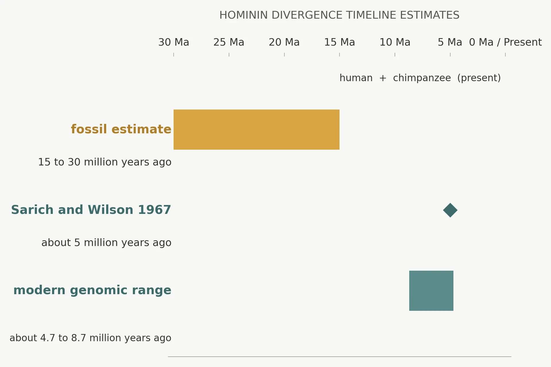
In December 1967, Sarich and Wilson published a result that told anthropologists their textbooks were wrong by ten million years or more. The reception in the literature was rough, and the argument ran for years. The two men had spent months in a laboratory measuring something that looked, to most people in the field, absurdly indirect: how strongly antibodies raised against human blood proteins reacted with the blood proteins of apes and monkeys. From those reactions they had built a molecular clock. And the clock said that humans and African apes had shared a common ancestor only about five million years ago.
That number landed like a small explosion. The fossil evidence of the day said something very different. The accepted story put the human line on its own path fifteen to thirty million years ago, deep in the Miocene, with plenty of time for a slow, dignified separation from the apes. A five-million-year split sounded reckless. It left almost no time for the changes that separate a chimpanzee from a person. It implied that the fossil record, the most respected witness in human origins, had been misread. Sarich and Wilson were accused, in print and in person, of trusting a laboratory trick over real bones in real rock.
The method itself was simple enough to explain to a stranger, and that simplicity was part of its power. They worked with serum albumin, a protein that floats in blood. When you inject human albumin into a rabbit, the rabbit makes antibodies that recognise that protein. Those antibodies will also react, more weakly, with albumin from a chimpanzee, still more weakly with albumin from a monkey, and weaker again with albumin from a more distant mammal. The strength of the reaction tracks how similar the proteins are. Sarich and Wilson measured that strength with a technique called quantitative micro-complement fixation, which sounds forbidding but amounts to a careful, repeatable way of asking: how much does this antibody still recognise that protein? The more the two proteins have diverged, the weaker the recognition. If proteins change at a roughly steady pace, the weakness of the reaction is a measure of time.
I first met this story as a student, in a lecture hall where the professor put the two numbers on the board side by side: fifteen to thirty million years from the fossils, about five million years from the blood. I remember the silence that followed, and then a hand going up at the back. "Which one is wrong?" the student asked. The professor smiled and said, "That is the question that kept a whole field busy for twenty years." I have carried that exchange with me ever since, because it captures what the molecular clock is for. It is not a gadget. It is a second witness, independent of fossils, that can be cross-examined against them. When the two witnesses disagree, something interesting is happening, and the job is to find out which one has been misunderstood.
1.1 December 1967: a graduate student and his professor vs. the fossil record
Sarich was a young researcher with a background in chemistry and a taste for argument. Wilson was a biochemist who had moved into evolution with the conviction that molecules could answer questions fossils could not. Together they chose serum albumin because it was abundant, easy to purify, and present in every primate they wanted to compare. They raised antibodies in rabbits, then tested those antibodies against albumin from humans, chimpanzees, gorillas, orangutans, Old World monkeys, New World monkeys, and more distant mammals. Each test gave a number: an immunological distance. Plot those distances against one another and a pattern emerges, a family tree drawn in chemistry rather than bone.
The logic was disarmingly direct. If albumin changes at a roughly constant rate, then the immunological distance between two species is proportional to the time since they last shared an ancestor. To turn a distance into a date, you need one anchor: a split whose date you think you know from fossils. Sarich and Wilson took the split between humans and Old World monkeys, which fossil evidence then placed at about thirty million years ago, and used it to calibrate everything else. The arithmetic pointed to a human and African ape split at about five million years, in the Pliocene. Their 1967 paper in Science, "Immunological time scale for hominid evolution", laid the result out plainly (Sarich and Wilson 1967).
The Berkeley evolution site still tells the story in the same plain terms: Sarich and Wilson "estimated that humans, chimpanzees, and gorillas shared a common ancestor only 5 million years ago — a much shorter length of time than was commonly accepted at the time" (UC Berkeley, Understanding Evolution). That sentence, read today, sounds tame. In 1967 it was a provocation. It said that a test tube could overrule a museum drawer.
1.2 What the fossils said: humans and apes split 15–30 million years ago
The fossil case was not foolish. It rested on a fossil called Ramapithecus, then read as a roughly fourteen-million-year-old human ancestor. If a creature that old already sat on the human side of the family tree, then the split from the apes had to be older still. Palaeontologists had built a coherent picture around that reading: an early Miocene separation, a long independent history for the human line, and a fossil record that seemed to confirm it at every turn. The confidence was understandable. Fossils are tangible. You can hold a jawbone. A protein reaction in a test tube feels, by comparison, like a rumour.
There was also a deeper worry, one that still echoes whenever a new dating method appears. Fossils date rocks. A fossil found in a layer of rock tells you that the animal lived when that rock formed, and radiometric dating can pin that down with real precision. Molecules, by contrast, date nothing directly. They give you a distance, and a distance only becomes a date when you borrow a date from somewhere else. To a palaeontologist in 1967, the molecular clock looked like a method that needed fossils to work, yet claimed to correct them. That tension was genuine, and it took years to resolve.
1.3 The answer from blood: about 5 million years
The calculation itself fits in a paragraph. Take the immunological distance between humans and Old World monkeys, and the fossil date for their split, about thirty million years. That gives you a rate: so much immunological change per million years. Now take the immunological distance between humans and chimpanzees, which is far smaller. Divide that smaller distance by the same rate, and you get a far shorter time: about five million years. Two years later, Wilson and Sarich consolidated the result across haemoglobin and albumin data and put "the most probable date at 4 to 5 million years" (Wilson and Sarich 1969). The number was stable. The method was not a fluke of one protein.
What made the result hard to dismiss was its internal consistency. The same rate that gave five million years for the human and ape split also gave sensible dates for other primate splits. The clock was not tuned to produce one surprising number; it produced a whole set of numbers that hung together. That coherence is what kept Sarich and Wilson going through the ridicule. A single odd result can be an artefact. A coherent pattern is harder to explain away.
1.4 The shockwave, and why it was eventually vindicated
The vindication came slowly, and it came from both sides. New fossil finds and a fresh look at old ones showed that Ramapithecus was not a human ancestor at all. It belonged on the orangutan line, and the fourteen-million-year pillar of the old chronology collapsed. Meanwhile, DNA sequencing, which barely existed in 1967, grew up and confirmed the young split again and again, gene after gene. The molecules had been right, and the fossils had been misread. The lesson was not that fossils are unreliable. It was that a single fossil, read one way, can mislead a whole field, and that an independent line of evidence is worth more than a second opinion from the same witness.
There is a twist, and it matters for everything that follows in this article. The modern estimates have drifted older than five million years. As we will see in §12, the honest range today is roughly 4.7 to 8.7 million years, depending on the method, with a major 2026 meta-analysis pushing the pooled estimate to about 7.3 to 8.7 million years. Sarich and Wilson were right that the split was young, and they were right that the old fossil reading was wrong. They were not right to the last decimal place, and nobody should expect them to have been. That drift is not a failure of the molecular clock. It is the clock doing what good instruments do: getting sharper as the data improve.
Hence, we suggest that apes and man have a more recent common ancestry than is usually supposed. — Sarich and Wilson, 1967, abstract of "Immunological time scale for hominid evolution", Science 158:1200–1203
That one sentence, quoted exactly as it appeared in the abstract, is the whole article in miniature. A careful measurement, a modest suggestion, and a field turned upside down. The question it leaves behind is the question this article answers: how can molecules tell time at all? To answer it, we need to understand what a molecular clock is, what makes it tick, and where it can be trusted and where it cannot.
2. What the Molecular Clock Actually Is
The molecular clock is a way of turning genetic differences into dates. Two species that shared a common ancestor long ago have had a long time to accumulate different mutations in their DNA. Two species that split recently have had less time, so their DNA is more similar. Count the differences, know roughly how fast differences accumulate, and you can estimate how long ago the split happened. That is the whole idea, and everything else in this article is detail, caveat, and worked example.
Penn State's S. Blair Hedges put it in the plainest terms I know: "Instead of measuring seconds, minutes and hours… the molecular clock measures the number of changes, or mutations, which accumulate in the gene sequences of different species over time" (Penn State). Nature Scitable states the hypothesis behind it just as plainly: "The molecular clock hypothesis states that DNA and protein sequences evolve at a rate that is relatively constant over time and among different organisms. A direct consequence of this constancy is that the genetic difference between any two species is proportional to the time since these species last shared a common ancestor" (Nature Scitable). Read those two sentences together and you have the definition. The rest is learning when "relatively constant" holds, when it does not, and what to do about it.
The molecular clock is especially valuable where fossils are scarce. Nature Scitable notes that it is a lifeline for organisms with a poor fossil record, such as flatworms and viruses. A virus leaves no fossil. A flatworm rarely does either. Without the molecular clock, their histories would be almost entirely guesswork. With it, we can date the emergence of HIV to the early twentieth century and the emergence of SARS-CoV-2 to November 2019, as we will see in §14. That range, from billions of years to a matter of weeks, is what makes the molecular clock one of the most versatile tools in evolutionary biology.
2.1 A clock that ticks in mutations, not seconds
Think of a wristwatch and a random process side by side. A wristwatch ticks at perfectly regular intervals, one second at a time, and you can trust it to the second. The molecular clock does not tick like that. Its ticks are mutations, and mutations happen at random. Some years a lineage picks up more changes than average; some years fewer. Over a short stretch, the count is noisy. Over millions of years, the noise averages out, and the total count grows roughly in step with time. That is why the word "relatively" in the Nature Scitable definition carries so much weight. The molecular clock is statistical, not mechanical.
A "tick" at the DNA level is a single change in a single letter of the genetic code: an A becomes a G, a C becomes a T, a short stretch is inserted or deleted. Most of these changes do nothing at all to the organism. They sit in stretches of DNA that do not code for protein, or they change a codon without changing the amino acid it specifies. Those silent changes are the molecular clock's best ticks, because nothing is actively removing them or favouring them. They accumulate the way dust accumulates on a shelf: steadily, quietly, and in proportion to time. Changes that alter a protein, by contrast, are subject to natural selection, which can speed them up or slow them down, and they make poorer clock ticks. We will return to that distinction in §9.
I once watched a graduate student stare at an alignment of two gene sequences on a screen, counting differences by eye, and mutter that it felt like counting raindrops to tell the time. That is not a bad description. One raindrop tells you nothing. A thousand raindrops over a season tell you something about the climate. The molecular clock works the same way: it needs enough ticks to drown out the randomness of any single one.
2.2 The core equation: time = genetic distance ÷ (2 × rate)
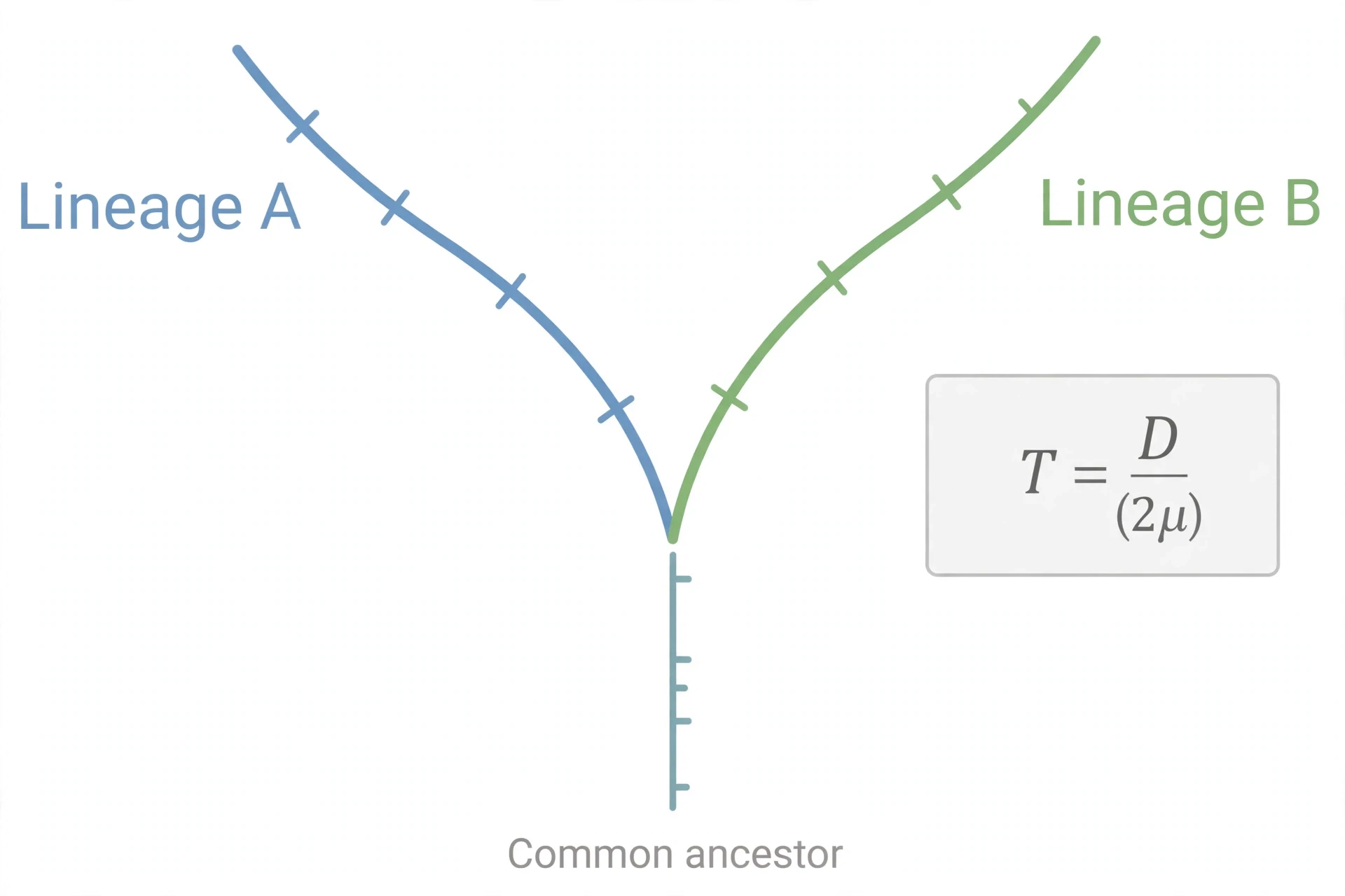
The article needs only one formula, and it is worth learning properly. Time equals genetic distance divided by twice the rate, written as T = D / (2μ). Here T is the divergence time, the number of years since two lineages last shared an ancestor. D is the genetic distance, the proportion of differences between the same gene in the two species. The Greek letter μ (mu) is the rate at which substitutions accumulate per site per year (Astronoo). The factor of 2 is the part people forget, and it matters. After two lineages split, each one accumulates changes independently. The total difference between them grows at twice the rate of either lineage alone, because both branches are ticking. Leave out the 2 and you will double the age of every split you date.
A toy example makes the arithmetic concrete. Suppose two species differ at 2 percent of the sites in a particular gene, so D is 0.02. Suppose the substitution rate for that gene is 1 percent per million years per lineage, so μ is 0.01 per million years. Then T equals 0.02 divided by 2 times 0.01, which is 0.02 divided by 0.02, which is 1 million years. The species split about a million years ago. Change the rate to 0.5 percent per million years and the same 2 percent difference means a split two million years ago. The distance is a fact you can measure. The rate is an estimate you must borrow or calibrate. The date is only as good as the rate, and that is why calibration, the subject of §7, is the heart of the whole enterprise.
2.3 Genetic distance: counting the differences
Genetic distance sounds abstract, but the procedure is concrete. Take the same gene from two species — say, the gene for cytochrome b, a protein in the mitochondria — and line the two sequences up side by side, letter by letter. Where the letters match, nothing has changed since the common ancestor, or the same change happened twice, which is rare over short times. Where they differ, at least one change happened on one branch or the other. Count the differences, divide by the total length, and you have a distance: a percentage, a proportion, a number you can feed into the equation.
Alignment is the quiet skill behind the whole method. Genes are not always the same length in two species. Insertions and deletions shift the letters out of register, and the alignment must decide which letters correspond to which. Get the alignment wrong and you count differences that are not real, or miss differences that are. For closely related species this is easy. For distant ones it becomes a careful, computer-assisted judgement. The molecular clock is only as honest as its alignment, and good studies say so openly.
2.4 Not the body clock: evolutionary clock vs. circadian clock
A short clarification belongs here, near the top, because the same phrase means two different things and search results mix them up freely. The molecular clock in this article is the evolutionary clock: a method for dating splits between species from DNA differences accumulated over millions of years. The other molecular clock is the circadian clock, the roughly 24-hour rhythm that governs sleep, hormone release, and metabolism in nearly every cell of your body. That clock is a real molecular machine, a transcription-translation feedback loop in which the CLOCK and BMAL1 proteins switch genes on, and the PER and CRY proteins switch them off again, once a day. It is a different concept from the evolutionary clock, and it answers a different question: what time of day is it inside a cell, not how many millions of years ago two species diverged (Circadian.news).
The confusion is understandable, and it is not the reader's fault. Both clocks are molecular. Both involve genes. But one ticks in hours and resets every morning, and the other ticks in mutations and never resets at all. If you came here looking for the body clock, you have the wrong article, and I would rather tell you that now than let you read ten thousand words before noticing. The FAQ in §19.7 returns to the distinction in full. A third clock, the epigenetic clock, which estimates age within a single lifetime from DNA methylation patterns, is also different from both, and §17.8 separates all three in one place.
What the molecular clock needs: the same gene compared in two species, a known or calibrated substitution rate, and at least one calibration point that ties a genetic distance to an absolute date.
What it does not need: fossils of the species themselves, a complete fossil record, or any assumption that the two species look different. Two species that look identical can still carry a measurable genetic distance, and the molecular clock will date their split anyway.
3. How the Clock Ticks: Mutations, Substitutions and Fixation
Three words get tangled together whenever people talk about the molecular clock, and untangling them is the key to understanding why the clock can work at all. A mutation is a change in DNA. A substitution is a mutation that has spread through an entire population until every individual carries it. Fixation is the process by which that spreading happens. Only substitutions count on the molecular clock, because only substitutions are shared by all members of a lineage and passed on to its descendants. A mutation that appears in one individual and vanishes with that individual leaves no trace in the species' DNA and tells us nothing about time.
The distinction matters because mutations are common and substitutions are comparatively rare. Every newborn human carries new mutations that neither parent carried in that form. Most of those mutations will vanish within a few generations, lost by chance when their carriers have no children, or have children who do not inherit that particular copy. A tiny fraction will spread, by luck or by advantage, until they are universal. The molecular clock counts the survivors, not the hopefuls.
3.1 Mutations happen every generation
DNA copying is astonishingly accurate and still imperfect. Every time a cell divides, its DNA must be copied, and the copying machinery makes occasional errors. Most errors are caught and repaired. A few slip through. In the germline, the cells that become eggs and sperm, those slipped-through errors become new mutations in the next generation.
The human numbers are now measured directly from families. The average human germline single-nucleotide mutation rate is about 1.2 × 10⁻⁸ per nucleotide per generation, with a range across trio studies of 0.96 to 1.29 × 10⁻⁸, corresponding to about 60 new mutations per newborn (review synthesising Roach et al. 2010 and others). Kong and colleagues, in a landmark 2012 trio study, found the same figure from the other direction: each newborn carries on average about 60 de novo mutations, and the number rises by about 1 to 2 per additional year of paternal age, while mothers contribute about 15 regardless of age (Kong et al. 2012). Campbell and colleagues, using a different method based on autozygosity, estimated a single-nucleotide mutation rate of 1.20 × 10⁻⁸ per base pair per generation, with a 95 percent confidence interval of 0.89 to 1.43 × 10⁻⁸, and found that CpG sites mutate about 9.5 times faster than non-CpG sites (Campbell et al. 2012). An earlier, pedigree-independent estimate by Nachman and Crowell (2000), comparing human and chimpanzee pseudogenes, gave a higher figure, about 2.5 × 10⁻⁸ per nucleotide per generation, or about 175 new mutations per diploid genome per generation — roughly double the modern pedigree-based rate, a gap that reflects the older fossil calibration and smaller ancestral population size assumed at the time (Nachman and Crowell 2000).
Sixty new mutations per child sounds like a lot until you set it against the scale of the genome. Three billion letters, sixty changes: the copying is 99.999998 percent accurate. Yet those sixty changes, generation after generation, are the raw material of the molecular clock. Over a million years, with a generation time of roughly twenty-five years, that is forty thousand generations and, in principle, millions of new mutations entering the population. Almost all of them vanish. The few that fix are the ticks we count.
For readers who want the background on how mutations arise and are inherited, the Sciory article on Genetics Explained: How Inheritance, Mutations, and Gene Expression Work covers the primer in full. What matters here is the rate, and the fact that it is measurable in living families, not just inferred from fossils.
3.2 Most mutations vanish; a few become substitutions
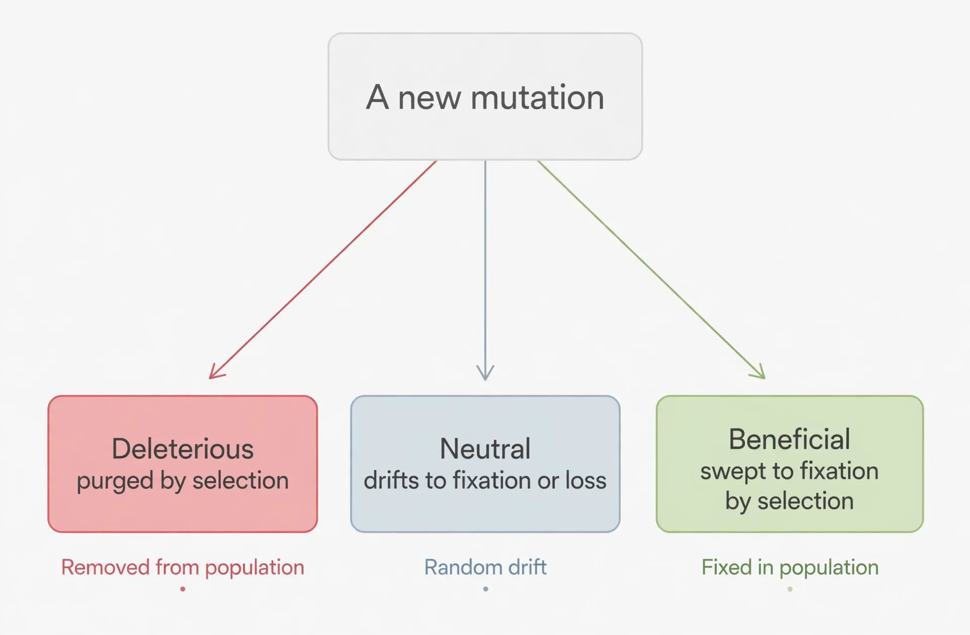
A new mutation starts life in a single individual, as one copy among two in a diploid genome. Its fate is decided by two forces: natural selection and genetic drift. Selection acts on mutations that affect survival or reproduction. A mutation that breaks a vital protein is purged quickly. A mutation that confers a real advantage can spread fast. Drift is the random sampling of genes from one generation to the next, and it governs the fate of mutations that selection cannot see: the neutral ones.
In a small population, drift is powerful. A neutral mutation can drift to fixation, meaning every individual ends up carrying it, purely by chance, the way a coin flipped enough times will eventually show a long run of heads. In a large population, drift is weaker, and a neutral mutation is more likely to vanish. The mathematics of this process is the subject of population genetics, and the Sciory article on Genetic Drift Explained: Bottlenecks and Founder Effects walks through it with worked examples. The point for the molecular clock is simple: fixation is a population process, not an individual one, and the rate at which neutral mutations fix is what sets the tick rate of the clock.
3.3 Why the substitution rate can equal the mutation rate
Here is the elegant result that makes the whole clock possible, and it belongs to Motoo Kimura. In a population, new neutral mutations appear at a rate that depends on the mutation rate and the population size: more individuals means more new mutations per generation. But each individual mutation has a smaller chance of fixing in a large population, because there are more copies to displace. Those two effects cancel exactly. The rate at which neutral mutations fix — the substitution rate — equals the mutation rate, regardless of population size. That is Kimura's key insight, previewed here and proved in §5. It means the molecular clock's tick does not depend on how many individuals there are, only on how often copying errors occur. A small population and a large population, with the same mutation rate, will accumulate substitutions at the same rate.
I remember the first time I worked through that cancellation on a whiteboard, and the quiet that fell over the room when the population size dropped out of the equation. It felt like a trick. It is not a trick. It is the reason a clock built from random events can be steady. The randomness of each mutation's fate averages out across the genome, and what remains is a rate set by chemistry, not by demography.
3.4 Per generation vs. per year: the unit problem
There is one more distinction to carry forward, because it explains a great deal of the variation we will meet in §10. Mutations happen per generation, when DNA is copied to make eggs and sperm. But we date splits in years. To convert a per-generation rate into a per-year rate, you need to know the generation time: how long, on average, between a parent's birth and the birth of its offspring. A mouse, with a generation time measured in months, copies its DNA many more times per million years than an elephant, with a generation time measured in decades. The mouse's clock, measured per year, ticks faster, even if the per-generation mutation rate is the same. This generation-time effect is one of the main reasons different species tick at different speeds, and it is why borrowing a rate from a distant relative is a mistake. The human mutation rate, measured in families, is a per-generation rate. The phylogenetic rate, inferred from splits dated by fossils, is a per-year rate. They are related, but they are not the same number, and confusing them has caused real errors in dating, as §12.4 will show.
4. The First Clockmakers: Zuckerkandl, Pauling and Haemoglobin (1962–1965)
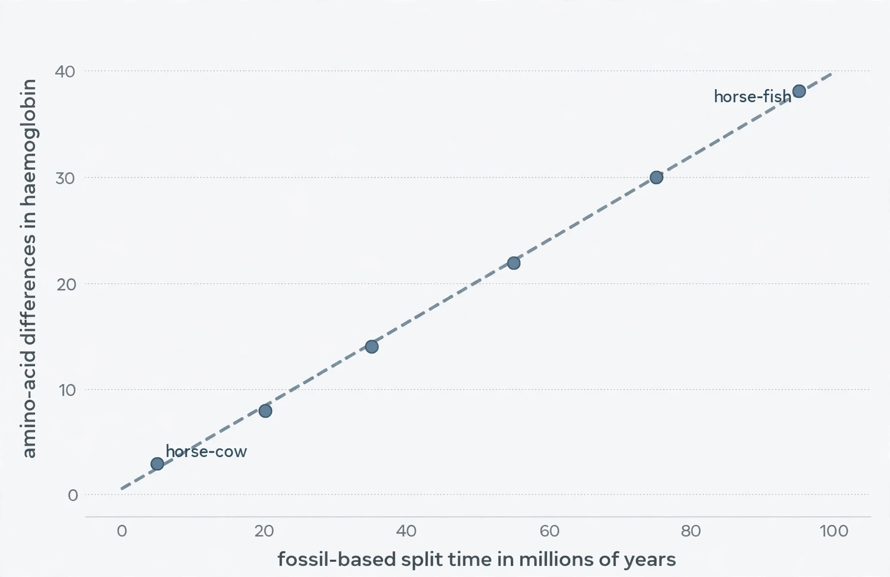
The molecular clock was not discovered in a single experiment. It was noticed, almost in passing, by two men studying a protein that had nothing to do with dating. Emile Zuckerkandl and Linus Pauling were interested in haemoglobin, the protein that carries oxygen in blood, and in what its variations could say about disease and evolution. What they found, in 1962, was a pattern nobody had expected: the number of amino-acid differences in haemoglobin between two lineages lined up, roughly, with the time since those lineages had split, as estimated from fossils. Horse and cow, close relatives, differed little. Horse and fish, distant relatives, differed a great deal. Plot the differences against the fossil dates and the points fell, more or less, on a straight line. That straight line was the first glimpse of the molecular clock (Zuckerkandl and Pauling 1962).
Pauling was already a towering figure, a Nobel laureate in chemistry with a second Nobel Peace Prize to come. Zuckerkandl was a younger biologist with a taste for big ideas. Together they had the confidence to generalise from a single protein to a principle: if haemoglobin changes at a roughly steady rate, then perhaps proteins in general do, and perhaps the differences between proteins carry a record of time. It was a bold leap, and it needed a mechanism. Neither man could say why the rate should be constant. They could only say that it looked constant. The mechanism would come from Kimura, six years later. But the observation came first, and observations have a way of outliving their explanations.
4.1 Caltech, 1962: haemoglobin differences line up with fossil time
The 1962 work appeared as a chapter, "Molecular disease, evolution, and genic heterogeneity", in a volume called Horizons in Biochemistry. Zuckerkandl and Pauling compared haemoglobin sequences across species and found that the count of amino-acid differences grew in step with fossil-based split times. The pattern was not perfect. No real data ever are. But it was clear enough to suggest a law-like regularity where nobody had expected one. Proteins were supposed to evolve under the messy, contingent pressure of natural selection, each lineage adapting to its own environment. Why should they change at anything like a constant rate? The data said they did, at least approximately, and the question of why became one of the most productive puzzles in evolutionary biology.
4.2 Margoliash and the equidistance surprise (1963)
A year later, Emanuel Margoliash added a second, stranger piece of evidence. He studied cytochrome c, a small protein involved in energy production in the mitochondria, and he found something that still stops me when I read it. The cytochrome c of a carp differs from the cytochrome c of a frog, a turtle, a chicken, a rabbit, and a horse by almost exactly the same amount: 13 to 14 percent in each case. Think about what that means. The carp lineage split from the frog lineage, the turtle lineage, the chicken lineage, and the mammal lineage at very different times in the deep past. Yet the carp is equally distant, in cytochrome c, from all of them. The only way that makes sense is if cytochrome c changes at a roughly constant rate in all those lineages, so that the distance from the carp to any land vertebrate depends only on the time since the carp lineage branched off, which is the same in every case. The fish is equally far from everything that came after it, because the molecular clock started ticking for all of them at the same moment: the moment the fish lineage went its own way.
Margoliash put the logic in a passage that deserves to be quoted exactly, because it is the clearest statement of the equidistance principle ever written:
It appears that the number of residue differences between cytochrome c of any two species is mostly conditioned by the time elapsed since the lines of evolution leading to these two species originally diverged. If this is correct, the cytochrome c of all mammals should be equally different from the cytochrome c of all birds. Since fish diverges from the main stem of vertebrate evolution earlier than either birds or mammals, the cytochrome c of both mammals and birds should be equally different from the cytochrome c of fish. Similarly, all vertebrate cytochrome c should be equally different from the yeast protein. — Emanuel Margoliash, 1963, "Primary Structure and Evolution of Cytochrome C", Proceedings of the National Academy of Sciences 50:672–679
The numbers backed the words. Carp cytochrome c differs from frog, turtle, chicken, rabbit, and horse by a very constant 13 to 14 percent. Bacterium versus yeast, wheat, moth, tuna, pigeon, and horse cytochrome c differ by 64 to 69 percent (Margoliash 1963). The constancy across such different animals is the point. It is hard to explain by adaptation, because a carp, a chicken, and a horse live in such different worlds. It is easy to explain by a clock: the same amount of time has passed since each of them last shared an ancestor with the carp.
4.3 1965: the "evolutionary clock" is named
In 1965, Zuckerkandl and Pauling gave the idea its name and its mathematics. Their paper, "Evolutionary Divergence and Convergence in Proteins", presented at the Evolving Genes and Proteins symposium and published in the symposium volume, called the pattern the "evolutionary clock" and derived its basic mathematical form (Zuckerkandl and Pauling 1965). They described its stochastic character, too: the clock ticks like a Poisson process, a random process in which events happen independently at a roughly constant average rate. That description matters, because it tells you what kind of precision to expect. A Poisson clock is not a wristwatch. Its ticks are random, and the count over a short interval is noisy. Over a long interval, the average asserts itself. Zuckerkandl and Pauling understood that from the start, and their honesty about the noise is one reason the field took them seriously.
They also recognised a condition that the clock depends on, one that is easy to overlook. For a molecular clock to exist, amino-acid changes must be limited almost exclusively to functionally nearly neutral changes. If most protein changes were strongly selected for or against, the rate would track the environment, not the time, and there would be no clock. That recognition, made in 1965, was the bridge to Kimura. The molecular clock needed neutral change, and Kimura would show that neutral change was abundant.
4.4 What they got right, and what they could not explain
Zuckerkandl and Pauling got the pattern right, the name right, and the mathematics right. What they could not explain was why the rate should be constant. Natural selection, as it was then understood, was supposed to drive change in fits and starts, fast when environments changed, slow when they were stable. A constant rate looked like a coincidence, or a artefact of averaging over many proteins and many lineages. The critics had a point, and the puzzle was genuine. The answer, when it came, did not come from haemoglobin or cytochrome c. It came from a population geneticist in Japan who was thinking about a different problem entirely: why evolution at the molecular level seemed far too fast for selection alone.
Species pair (haemoglobin / cytochrome c) | Approximate amino-acid difference | Fossil-based split time (schematic) |
|---|---|---|
Carp vs. frog, turtle, chicken, rabbit, horse (cytochrome c) | 13–14% in each case | Same deep split from the fish lineage in each case — hence equal distance |
Bacterium vs. yeast, wheat, moth, tuna, pigeon, horse (cytochrome c) | 64–69% | Far older divergence, hence far larger difference |
Horse vs. cow (haemoglobin) | Small | Recent split, tens of millions of years |
Horse vs. fish (haemoglobin) | Large | Ancient split, hundreds of millions of years |
The table is schematic, not a laboratory notebook. Its purpose is to show the pattern Zuckerkandl, Pauling, and Margoliash saw: difference grows with time, and equal times give equal differences, even across animals as different as a carp and a horse. That pattern, once seen, could not be unseen.
5. Why the Clock Can Tick: Kimura's Neutral Theory (1968) and King & Jukes (1969)
The puzzle Zuckerkandl and Pauling left behind was a problem of speed. If every molecular change had to be driven by natural selection, then evolution at the molecular level was happening far too fast. J. B. S. Haldane had calculated, in 1957 (Haldane 1957), an upper limit on how fast adaptive evolution could proceed: a population can only afford to replace so many genes per generation before the cost in deaths and failed reproductions becomes unbearable. The substitution rates implied by the protein data blew straight past that limit. Something was wrong with the assumption, not with the data. Most molecular change, Motoo Kimura argued, was not adaptive at all.
Kimura was a population geneticist at the National Institute of Genetics in Japan, a quiet, mathematically formidable thinker who had spent years working out the theory of genetic drift. In 1968 he published a short paper in Nature, "Evolutionary rate at the molecular level", that changed the field. Its central sentence is worth quoting in full, because it is the hinge on which the molecular clock turns: "Calculating the rate of evolution in terms of nucleotide substitutions seems to give a value so high that many of the mutations involved must be neutral ones" (Kimura 1968). If the rate is too high for selection, and the changes are happening anyway, then the changes must be neutral: invisible to selection, governed by drift, and free to accumulate at the mutation rate.
5.1 The problem: evolution seemed far too fast for selection alone
Haldane's dilemma, as it came to be called, was a cost argument. Every time a beneficial mutation spreads through a population, individuals who lack it are, by definition, less fit, and some of them fail to reproduce. There is a limit to how much of that a population can bear in each generation. Kimura took the substitution rates extrapolated from three proteins and showed that they far exceeded Haldane's upper limit for adaptive evolution (Oxford Bibliographies, Neutral Theory). The conclusion was forced: most substitutions must be neutral. The field had been assuming that molecular evolution was natural selection writ small. Kimura showed that it was mostly drift writ small, with selection acting on a minority of changes.
5.2 Kimura 1968: most molecular change is neutral
The neutral theory, as Kimura framed it, has a clean core. Most genetic differences between species, and most polymorphisms within species, are selectively neutral and result from mutation and genetic drift. The theory applies only at the molecular level and is compatible with phenotypic evolution by natural selection (Neutral theory of molecular evolution). That last clause matters enormously, and it is the part most often dropped by critics. Kimura was not saying that natural selection does not shape bodies, behaviours, or beaks. He was saying that at the level of DNA letters and amino acids, most changes do not affect the organism enough for selection to notice, and those changes accumulate by chance at a steady rate. The molecular clock ticks because selection is not interfering.
The key quantitative result, previewed in §3.3, is that the neutral substitution rate equals the mutation rate. Nature Scitable states it directly: Kimura showed the neutral substitution rate, the fixation rate, equals the mutation rate, so if the mutation rate is constant across species, the substitution rate, the clock's tick, is constant too (Nature Scitable). That equality is what turns a random process into a usable clock. The mutation rate is set by chemistry, the fidelity of DNA copying, and chemistry does not change much from one mammal to the next. So the molecular clock ticks at a similar rate in different lineages, at least to a first approximation. The approximations, and their failures, fill §9 and §10.
5.3 King & Jukes 1969: "Non-Darwinian evolution"
A year later, Jack King and Thomas Jukes published an independent argument in Science under a title designed to provoke: "Non-Darwinian evolution" (King and Jukes 1969). Their case was built from protein data, not population-genetic theory, but it reached the same conclusion: most molecular change is neutral, and selection cannot explain the rate. The title caused a storm, because it sounded like an attack on Darwin. It was not. King and Jukes were explicit that natural selection shapes adaptation. What they denied was that selection drives most molecular change. The storm was partly a misunderstanding, and partly a genuine shock at how much of evolution, at the molecular level, is driven by chance. The Sciory article on Natural Selection Explained: How Evolution Really Works sets out the selection side of the story in full, and the two articles belong together: selection shapes bodies, drift fills in the molecular details.
5.4 Nearly neutral: Ohta's refinement
The strict neutral theory, in its original form, has softened over time, and it is important to say so. Tomoko Ohta, Kimura's colleague, proposed the nearly neutral theory (Ohta 1973): many mutations are not perfectly neutral but slightly deleterious, harmful enough that selection can remove them in a large population, but weak enough that drift can fix them in a small one. Population size therefore matters after all, not for perfectly neutral mutations, where it cancels out, but for the large class of slightly deleterious ones. In small populations, more slightly harmful mutations drift to fixation, and the molecular clock ticks faster. In large populations, selection purges them, and the molecular clock ticks slower. The strict neutral theory has generally fallen out of favour as a complete explanation, with the nearly neutral theory and selection also invoked, but neutral theory remains the standard null model for molecular evolution. That is the right way to think about it: a null model, a starting expectation, against which real data can be tested. When a gene ticks faster or slower than the neutral expectation, that deviation is information, not failure.
5.5 What neutral theory does NOT say
Let me be direct about a misconception I hear often, because it does real damage. Neutral theory does not say that evolution is random, or that natural selection is unimportant, or that adaptation is an illusion. It says that at the molecular level, most changes are neutral. The beak of a finch, the wing of a bat, the eye of an octopus: those are products of selection, shaped over millions of years by the relentless filtering of variation. The silent change in the third position of a codon, which does not alter the amino acid at all, is not. Both statements are true at once. The molecular clock works because the second kind of change is abundant. It does not work in spite of selection; it works alongside it, measuring time with the changes selection ignores.
Deleterious: a new mutation harms its carrier. Selection purges it, usually within a few generations. It never becomes a substitution, and it never ticks the clock.
Neutral: a new mutation does nothing selection can see. It drifts, and a small fraction fix by chance. Those fixations are the clock's ticks.
Beneficial: a new mutation helps its carrier. Selection sweeps it to fixation quickly. These are rare at the molecular level, and they tick the clock faster than the neutral rate while they last, which is one reason a single gene can mislead.
6. Reading the Clock: How Scientists Actually Date a Split
So far the molecular clock has been an idea. Now it becomes a procedure. Dating a split is not a matter of plugging two numbers into a formula and printing a date. It is a sequence of choices, each of which can go wrong, and good studies are explicit about every one of them. The steps below are the standard workflow, and they are worth walking through slowly, because once you have seen them, you will never again read a headline date without asking how it was obtained.
The first thing to notice is how ordinary the steps are. There is no single machine that dates a split. There is a gene, an alignment, a rate, a calibration, and a cross-check. Each step is a judgement call, and the error bars on the final date are a record of how uncertain those judgements were. A study that reports a date without error bars is not being precise. It is hiding its uncertainty.
6.1 Step 1 — pick the right gene
Not every gene is a good clock for every question. A gene that changes fast is useful for recent splits, where you need enough differences to count, but useless for ancient ones, where it will have changed so many times that the signal is saturated. A gene that changes slowly is useful for deep splits, where you need a signal that has survived hundreds of millions of years, but useless for recent ones, where it may not have changed at all. The choice of gene is the choice of clock speed, and it must match the depth of the question.
Conserved genes, the ones whose proteins are so important that almost any change breaks them, tick slowly. They are the molecular clocks for deep time: the origin of animals, the split between major groups. Fast genes, especially mitochondrial genes in animals, tick quickly. They are the molecular clocks for recent time: splits within the last few million years, population histories, the emergence of a virus. A study that uses a fast gene to date a deep split, or a slow gene to date a recent one, will get a wrong answer, and the error will not announce itself. The gene must fit the question, the way a ruler must fit the object being measured.
6.2 Step 2 — align and count
Once the gene is chosen, the sequences from the two species are aligned, letter by letter, so that corresponding positions line up. The count of differences is the raw genetic distance. But the raw count is not the true count. Over long times, the same site can mutate twice: an A becomes a G, then the G becomes a T, and the final comparison shows one difference where two changes happened. Or an A becomes a G and then back to an A, and the comparison shows no difference where two changes happened. Raw counts underestimate deep divergences because of these multiple hits, and substitution models exist to correct for them. The simplest, the Jukes-Cantor model, assumes every change is equally likely and corrects the raw distance upward by an amount that grows with the distance itself. More elaborate models allow for the fact that some changes, such as transitions between similar bases, are more common than others. The correction is not a fudge. It is a statistical adjustment based on what we know about how mutations happen, and without it, deep dates come out systematically too young. We return to the problem in full in §11, under the name saturation.
6.3 Step 3 — apply the rate, get a date (with error bars)
With a corrected distance and a rate, the equation from §2.2 gives a date. The rate, remember, is not measured in the study itself. It is borrowed from a calibration, or estimated alongside the date in a joint analysis. Either way it carries uncertainty, and that uncertainty propagates into the date. A date reported as a single number, without a range, is a date with its uncertainty removed. Good studies report a range: a confidence interval, or in Bayesian analyses, a credibility interval, usually a 95 percent interval that says, in effect, the true date lies in this range with 95 percent probability under the model used. The width of that interval is information. A narrow interval means the data constrain the date tightly. A wide interval means they do not, and the honest response is to say so.
A worked example, using the bird numbers from §7, makes the step concrete. Two bird species differ at 2 percent of the sites in cytochrome b. The cytochrome b rate in birds is about 1 percent per lineage per million years. Applying T = D / (2μ), the split is about 1 million years ago. But the rate is not exactly 1 percent. Some bird lineages tick faster, some slower, and the calibration itself has error bars. The honest date is therefore not "1 million years" but "about 1 million years, with a range that reflects the uncertainty in the rate and the calibration". That phrasing is longer and less headline-friendly. It is also true, and the difference matters.
6.4 Step 4 — cross-check with a second gene and a second method
No serious dating rests on a single gene. Different genes tick at different rates, and a single gene can be misleading for reasons that have nothing to do with time: selection on that gene, a burst of change in one lineage, a hybridisation event that moved the gene between species. The standard practice is to date the same split with several genes, preferably from different parts of the genome, and to check that they agree. If they do, confidence rises. If they do not, the disagreement is itself informative: it points to the gene or the lineage that is behaving unusually.
The same logic applies to methods. A date obtained with a strict clock can be checked with a relaxed clock. A date obtained with one set of fossil calibrations can be checked with another. A date obtained from DNA can be checked against a date obtained from the fossil record, or from a biogeographic event. The molecular clock is at its most convincing not when a single analysis gives a clean number, but when independent analyses converge on the same range. That convergence is what we will see in the human story in §12, and its absence is what we will see in the unresolved cases in §16.
What, then, is a "split"? The word is used loosely in popular writing, and it deserves a precise meaning here. A split is the moment two populations stop exchanging genes and go their separate evolutionary ways. It is a population event, not a fossil event, and the molecular date for a split is the date of genetic isolation, which is always older than the first fossil of either descendant group. The Sciory article on Speciation Explained: How New Species Form explains how that isolation happens, and why a split is a process, not an instant. Keep that in mind whenever a molecular date and a fossil date disagree by a few million years: some of that gap is expected, because the two methods date different things.
Gene | Genetic difference | Rate (per lineage) | Date ± uncertainty |
|---|---|---|---|
Bird cytochrome b (illustrative) | 2% divergence | About 1% per million years | About 1 million years, with a range reflecting rate and calibration uncertainty |
Bird cytochrome b (illustrative) | 10% divergence | About 1% per million years | About 5 million years, before correction for multiple hits; corrected distance gives an older date |
Primate mitochondrial DNA (illustrative) | 2% divergence | About 1% per lineage per million years (2% pairwise; classic rough calibration) | About 1 million years, as a rough guide only |
The table is deliberately labelled illustrative. The bird rate is the real Weir and Schluter figure, from §7. The dates are what the equation gives when you feed it those numbers. The lesson is not the numbers themselves but the pattern: the same distance means different dates under different rates, and the uncertainty in the rate is the uncertainty in the date.
7. Calibrating the Clock: Fossils, Rocks and Islands
The molecular clock alone gives only relative time. That sentence is worth repeating, because it is the single most misunderstood fact about the method. The molecular clock can tell you that one split is twice as old as another. It cannot tell you that either split happened a specific number of millions of years ago. For absolute dates, you need a calibration: an independent piece of information that ties a genetic distance to a known date. Without calibration, the molecular clock is an odometer without a speedometer reading, a ruler without units.
Nature Scitable gives the analogy that every student remembers: knowing two sequences differ by 5 percent cannot tell you whether they diverged at 1 percent per million years over 5 million years or 5 times faster over 1 million years. That, the page says, is "equivalent to trying to determine the average speed of a car merely by looking at its odometer" (Nature Scitable). The odometer tells you how far the car has travelled. It does not tell you how fast it went, or how long the journey took. A fossil calibration is the equivalent of knowing that the car passed a particular town at a particular time. With enough such landmarks, you can reconstruct the speed, and then the whole journey.
7.1 Why calibration is unavoidable
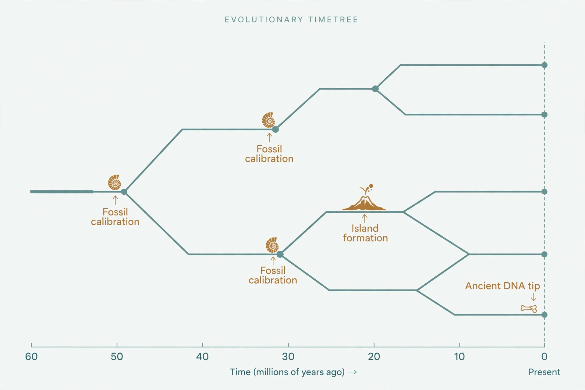
Rate and time are confounded. A large genetic distance can mean a long time at a slow rate, or a short time at a fast rate, and the DNA alone cannot tell you which. Every molecular date therefore rests on an assumption about the rate, and that assumption must come from outside the DNA. The most common source is fossils. The second is geology: a land bridge forming, an island emerging from the sea, a mountain range rising and splitting a species' range. The third, increasingly important, is ancient DNA: a genome from a directly dated fossil or subfossil, whose age is known from radiocarbon or stratigraphy. Each source has its own strengths and its own traps, and the best studies use several at once.
7.2 Fossil calibration (node dating)
Fossil calibration, also called node dating, works by attaching a fossil to a node, a branching point, on the evolutionary tree. The logic is simple and strict. If a fossil belongs to a particular group, then that group must be at least as old as the fossil. The fossil gives a minimum age for the node. It cannot give a maximum age, because the group could be older than its oldest known fossil, and almost always is. Fossils are rare. A lineage must become abundant and widespread enough to leave a fossil, and that fossil must survive, be found, and be correctly identified. The first fossil of a group is therefore a late witness, not an early one.
That asymmetry shapes every fossil calibration. A good calibration treats the fossil age as a minimum and allows the true split to be older, sometimes much older. Modern methods do this formally, with probability distributions that put a hard floor at the fossil age and a long tail stretching into the past. A bad calibration treats the fossil age as the split age, and dates everything too young. Cunningham and colleagues put the principle clearly: fossil dates give minimum ages for a group, because the oldest fossil is at best the time a lineage had become abundant and widespread enough to fossilise, while the molecular date, the genetic isolation time, is necessarily earlier (Cunningham et al. 2017). For readers who want the fossil side of the story, the Sciory article on The Fossil Record Explained: How Fossils Form explains how fossils form, why they are rare, and why the record is biased toward some animals and environments and against others. The fossil dates themselves rest on radiometric dating of the surrounding rocks, which the Sciory article on Radioactivity Explained: Half-Life and Nuclear Decay explains in full.
7.3 Biogeographic calibration
Geology can calibrate a clock when a geological event splits a population. When a land bridge forms or breaks, when an island rises from the sea, when a mountain range lifts and divides a species' range in two, the populations on either side stop exchanging genes. If the geological event can be dated, by radiometric dating of the rocks, then the genetic split can be dated to the same event. Island formation is the classic case. A volcanic island emerges sterile, is colonised once, and the colonists then evolve in isolation. The age of the island is a maximum age for the colonisation, and a minimum age for the subsequent radiation. Land bridges work the same way in reverse: the formation of the Panama land bridge, about three million years ago (full closure around 2.8 million years ago, after a gradual shoaling), split marine populations on the Atlantic and Pacific sides, and the genetic distance between those populations, divided by the known time, gives a rate.
Biogeographic calibrations are elegant, but they carry a risk. The geological event and the genetic split do not always coincide. A population can cross a new land bridge long after it forms, or survive on both sides of a new mountain range for millions of years before finally separating. The calibration assumes a coincidence that must be argued, not assumed. Good studies argue it explicitly, and they use several independent biogeographic events, not one.
7.4 Tip dating and ancient DNA
Tip dating is the newest calibration method, and in some ways the most direct. Instead of attaching a fossil to a node deep in the tree, you attach a directly dated genome to a tip, a living or extinct sample at the end of a branch. An ancient genome from a 35,000-year-old wolf, or a 1959 sample of HIV, has a known age, from radiocarbon dating or from the date the sample was collected. That age anchors the branch it sits on, and the anchor propagates through the tree. The Taimyr wolf genome, discussed in §14, is the textbook example: a 35,000-year-old wolf genome recalibrated the dog domestication clock by showing that the mutation rate was slower than assumed, and pushed the dog and wolf split earlier than previous estimates had placed it.
Ancient DNA has transformed calibration because it provides dates that are not minimum ages but actual ages. A fossil gives you a floor. An ancient genome gives you a point. The difference is the difference between knowing a building is at least a century old and knowing it was built in 1923. As ancient genomes accumulate, from humans, animals, and pathogens, the molecular clock's calibrations are getting sharper, and the error bars on recent dates are shrinking.
7.5 The gold standard in action: Weir & Schluter's birds (2008)
The best-known calibration study in the field is also one of the most careful. Jason Weir and Dolph Schluter, in 2008, set out to calibrate the avian cytochrome b clock, the workhorse gene for bird dating. They gathered 90 calibrations: dated fossils, land-bridge ages, island formation ages, and mountain uplift ages. Then they did something that takes discipline: they tested each calibration against the others and discarded 16 as inconsistent. Sixteen out of ninety is a substantial cull, and it is the reason the study is trusted. A calibration that disagrees with all the others is more likely to be wrong than to be a lone voice of truth.
From the remaining 74 calibrations, Weir and Schluter estimated a rate of about 1 percent sequence divergence per lineage per million years, meaning two bird species diverge at about 2 percent per million years. That is the famous "2 percent rule" for birds, and it has been used to test whether many modern songbird species originated during glacial cycles over the past 250,000 years (Weir and Schluter 2008). The rule is real, and it is useful. It is also lineage-specific, and Weir and Schluter were explicit about its limits. Bird rates vary. Many lineages sit near the 1 percent average, but some evolve more than 4 times faster than others, and Weir and Schluter found no correlation with body mass. Borrow the 2 percent rule for a bird lineage that ticks at 4 percent per million years and you will date its splits at half their true age. The rule is a starting point, not a universal constant.
A related classic deserves a mention here because it still appears in textbooks. The primate mitochondrial DNA calibration of about 2 percent per million years, from Brown and colleagues in 1979, is still sometimes used for mammals and birds, though it is rough (Nabholz and colleagues). Rough is the right word. It is a useful first guess and a poor final answer.
Use multiple calibrations. One calibration can be wrong. Several, from different sources, that agree are hard to dismiss.
Never treat a fossil age as the split age. A fossil is a minimum. The split is older, sometimes much older.
Never borrow a rate from a distant relative. A rate measured in one lineage is an estimate for that lineage. The next lineage over may tick at a different speed.
Discard inconsistent calibrations openly. Weir and Schluter discarded 16 of 90 and said so. That transparency is what makes their rate believable.
Report the uncertainty. A calibration with error bars produces a date with error bars. Hiding the first does not remove the second.
8. Strict Clocks vs. Relaxed Clocks
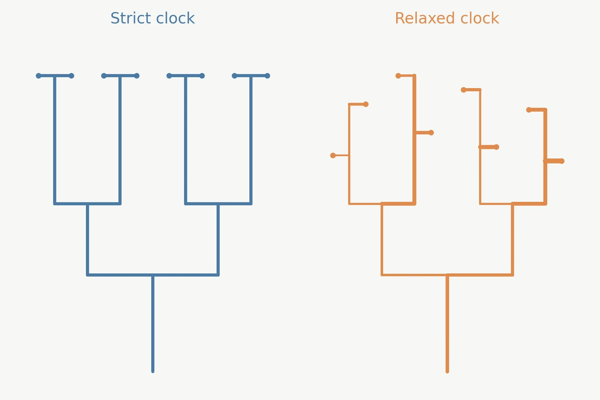
The early molecular clock was a strict clock: one rate, applied to every branch of the tree, for all time. It was elegant, and it was mostly wrong. The data that accumulated through the 1980s and 1990s showed, again and again, that rates vary: between genes, between lineages, and over time within a lineage. The field's response was not to abandon the molecular clock. It was to build better clocks, ones that let the rate vary and that report the uncertainty that variation creates. That move, from strict to relaxed clocks, is the most important methodological shift in the history of molecular dating, and it is the reason modern dates carry credibility intervals instead of false precision.
8.1 The strict clock: elegant, and mostly wrong
A strict clock assumes that the substitution rate is the same on every branch of the tree. That assumption is testable, and it fails often. Nature Scitable puts it bluntly: the strict-clock assumption is "too simplistic, because rates of molecular evolution can vary significantly among organisms" (Nature Scitable). The strict clock still works in limited settings: closely related species, over short timescales, where the rate has not had time or opportunity to vary much. A study of a recent radiation, a group of species that split within the last few million years, can often use a strict clock safely. A study of the whole tree of life cannot. The strict clock is a special case, not the general rule, and treating it as the general rule was the field's first systematic error.
8.2 Relaxed clocks I: rates vary around an average
The first family of relaxed clocks lets each branch have its own rate, drawn from a distribution around an average. The most widely used version is the uncorrelated lognormal model, in which each branch's rate is drawn independently from a lognormal distribution. "Uncorrelated" means that a fast branch does not predict a fast daughter branch. The rate on each branch is its own draw, independent of its neighbours. That sounds like giving up: if every branch can have its own rate, how can you date anything? The answer is that the rates are not free. They are constrained by the calibrations and by the assumption that they cluster around an average. The model trades the false precision of a single rate for the honest uncertainty of a distribution, and the resulting dates carry wider, but more trustworthy, intervals.
8.3 Relaxed clocks II: rates themselves evolve
The second family of relaxed clocks assumes that rates are correlated: a fast lineage tends to produce fast descendants, because the biological properties that set the rate, body size, metabolic rate, generation time, DNA repair efficiency, are inherited. These are autocorrelated models, in which the rate evolves along the tree the way a trait evolves. The two families make different assumptions, and they can give different dates. Which one is right depends on the group being studied, and the honest approach is to try both and see whether the dates agree. When they do, confidence rises. When they do not, the disagreement is a signal that the rate variation is not well understood, and the dates should be reported with that caveat attached.
8.4 BEAST and the Bayesian revolution
The tool that made relaxed clocks practical is BEAST, Bayesian Evolutionary Analysis by Sampling Trees, introduced by Alexei Drummond and Andrew Rambaut in 2007 (Drummond and Rambaut 2007). BEAST, and the relaxed-clock framework it implements, described by Drummond and colleagues in 2006 (Drummond et al. 2006), does not produce a single date. It produces a distribution of dates, sampled from all the trees and rates that are consistent with the data and the calibrations. The output is a credibility interval, usually a 95 percent highest posterior density interval, which says where the true date probably lies. That is a different kind of answer from a strict-clock date, and a better one. It is an admission of uncertainty, built into the method, not bolted on afterwards.
How well do relaxed clocks work? A simulation study by Battistuzzi and colleagues in 2010 gives a clear answer. Relaxed-clock methods perform well when the assumed lineage-rate model matches the true one: 95 percent credibility intervals contain the true time at least 95 percent of the time in simulations. When the model is wrong, the coverage drops to 83 percent. Composite intervals from BEAST and MultiDivTime contain the true time at least 97 percent of the time (Battistuzzi et al. 2010). Those numbers are reassuring and sobering in equal measure. The methods work when their assumptions hold, and they degrade gracefully, not catastrophically, when they do not. The lesson is to check the assumptions, not to trust the software blindly.
One modern framework deserves a paragraph of its own. The fossilised birth-death model (Heath et al. 2014) treats fossils not as fixed calibration points but as part of the same process that generates the tree: lineages are born, they die, and they leave fossils with a certain probability. Fossils are sampled alongside living species, and their ages inform the dates directly. That is a more realistic treatment than node dating, because it models the fossil record's incompleteness instead of pretending a fossil age is a hard boundary. It is also more demanding, because it needs a model of fossilisation and sampling. It is, at the time of writing, the state of the art for studies that have enough fossils to use it, and it is the direction the field is moving.
8.5 Local clocks: a middle path
Between the strict clock and the fully relaxed clock sits the local clock: different rates for different parts of the tree. A study might assign one rate to primates, another to rodents, and a third to bats, on the grounds that each group is internally homogeneous but different from the others. Local clocks are a compromise. They are simpler than fully relaxed models, and they are easier to interpret: the rate for each group is a number you can report and discuss. They are also riskier, because the boundaries between groups are chosen by the researcher, and a wrong boundary can bias the dates. Like every method in this section, they are a tool, not a truth.
Clock model | Assumption | When to use it | Risk |
|---|---|---|---|
Strict clock | One rate for the whole tree | Closely related species, short timescales | False precision when rates vary; dates biased if the rate is wrong |
Relaxed clock (uncorrelated) | Each branch rate drawn independently around an average | Most modern dating; rate variation expected but not inherited | Wide intervals; sensitive to the assumed rate distribution |
Relaxed clock (autocorrelated) | Rates evolve along the tree; fast lineages beget fast descendants | Groups where rate is tied to inherited biology, such as body size | Wrong if rates are not actually inherited; can understate uncertainty |
Local clock | Different rates for different parts of the tree | Groups with clear rate shifts between clades | Boundaries chosen by the researcher; a wrong boundary biases dates |
A 2026 review of the field summarises the shift in one sentence: molecular clocks have evolved "from relatively simple strict-rate assumptions into a diverse set of statistical frameworks that include strict, relaxed, local and time-dependent models". The same review states the conclusion that every section of this article has been building toward: "There is no universal molecular clock, and, in fact, not even a single molecular clock exists for an organism" (Soares and Rito 2026). That is not a counsel of despair. It is a description of a mature science, one that has replaced a simple idea with a family of models and learned to report what it does not know.
9. Why Different Genes Tick at Different Speeds
There is no single molecular clock. That statement, which the 2026 review makes as its central conclusion, is worth sitting with. Every gene is a different clock. Every genome is a different clock. The same gene in two species can tick at different speeds, and the same species can carry genes that tick at speeds differing by a factor of ten or more. The molecular clock is not a single instrument. It is a workshop full of instruments, each with its own rate, and the skill of molecular dating is choosing the right one for the question at hand.
9.1 Synonymous vs. nonsynonymous changes
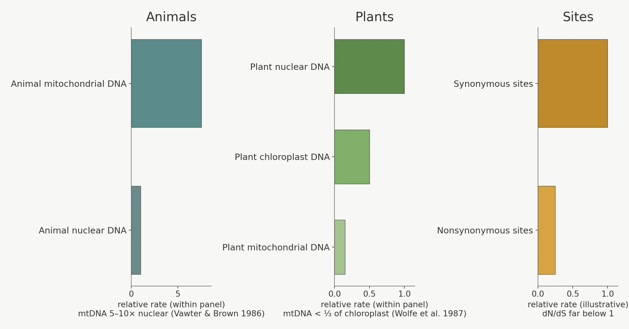
The most fundamental split is between synonymous and nonsynonymous changes. A synonymous change alters a DNA letter without altering the amino acid it codes for, thanks to the redundancy of the genetic code. It is invisible to selection at the protein level, and it accumulates at close to the neutral rate. A nonsynonymous change alters the amino acid, and therefore potentially the protein, and selection notices. Most nonsynonymous changes are harmful and are purged. A few are beneficial and sweep. The net effect is that nonsynonymous sites tick far slower than synonymous sites, because most of their changes are removed before they can fix.
The ratio of the two rates, called dN/dS, is a standard diagnostic. A dN/dS near 1 means the gene is evolving neutrally: nonsynonymous changes fix as readily as synonymous ones. A dN/dS far below 1 means purifying selection is at work, purging most protein-changing mutations. A dN/dS above 1, rare and interesting, means positive selection is driving protein change. For dating, synonymous sites are usually the better clock, because they tick faster and more neutrally. But they also saturate faster, because they change so often that the same site is hit twice. The choice between synonymous and nonsynonymous sites is a trade-off between speed and longevity, and good studies use both and compare the answers.
9.2 Mitochondrial vs. nuclear DNA in animals
In animals, mitochondrial DNA ticks far faster than nuclear DNA. The classic figure, from Vawter and Brown in 1986, is that vertebrate mitochondrial DNA evolves 5 to 10 times faster than vertebrate single-copy nuclear DNA, a disparity they took as evidence against a generalised molecular clock (Vawter and Brown 1986). Textbooks often round the figure to about 10 times faster, and that rule of thumb is useful for recent population splits and migrations, where you need a fast clock to see any differences at all. But it is a rule of thumb, not a measurement, and it varies by gene and by lineage.
Why is mitochondrial DNA faster? The mitochondria are the cell's power stations, and they generate reactive oxygen species as a by-product of making energy. The mitochondrial genome sits in the line of fire, exposed to that damage, and it has less efficient repair than the nuclear genome. It is also inherited maternally, without recombination, which means it behaves as a single linked unit. Those properties make it a superb clock for recent splits, and a poor clock for deep ones, where its speed becomes a liability. It saturates, it is prone to selection on its energy genes, and its maternal inheritance means it tracks only the female line. The human mitochondrial story in §12.3, including Mitochondrial Eve, is a mitochondrial story, and its limits are mitochondrial limits.
9.3 The plant exception: three genomes, three speeds
Plants reverse the animal pattern, and the reversal is a useful reminder that there is nothing universal about the rates. Wolfe, Li, and Sharp showed in 1987 that the silent substitution rate in plant mitochondrial DNA is less than one-third that in chloroplast DNA, which in turn evolves only about half as fast as plant nuclear DNA (Wolfe et al. 1987). In plants, mitochondrial DNA is the slowest genome, nuclear DNA the fastest, and chloroplast DNA in the middle. That is the opposite of the animal pattern, where mitochondrial DNA is the fastest.
The reason is not fully settled, but the leading explanation is that plant mitochondria have unusually efficient DNA repair and low mutation rates, while their nuclear genomes, exposed to the same environmental mutagens as any other genome, tick at a more ordinary pace. Whatever the cause, the practical consequence is clear: a dating method built for animals cannot be transplanted to plants without rethinking the rates. The Sciory article on Plant Evolution Explained: From Algae to Flowering Plants covers the plant story in full, and the three-genome pattern is one of its most surprising details.
9.4 Protein constraint: cytochrome c vs. fibrinopeptides
The same logic applies within the nuclear genome. Different proteins evolve at very different rates, a fact already known by the early 1970s. The rate depends on functional constraint: how much of the protein can change without breaking it. Cytochrome c, which sits at the heart of energy production and interacts with many other proteins, is highly constrained. Almost any change breaks something, so almost every change is purged, and the protein ticks slowly. Fibrinopeptides, short peptides that are clipped off during blood clotting and serve no function afterwards, are almost unconstrained. Changes accumulate freely, and the peptides tick fast. Histones, the proteins that spool DNA, are among the slowest of all, because their structure is so critical that even a single change can be lethal. The range between the slowest and fastest proteins spans orders of magnitude.
That range is why the choice of gene matters so much. A study that dates a deep split using fibrinopeptides will saturate and fail. A study that dates a recent split using histones will find no differences at all and conclude, wrongly, that the split was yesterday. The gene must match the depth, and the researcher must say why the chosen gene fits.
9.5 Which gene for which question
The practical guide is simple to state and easy to get wrong in practice. For recent splits, within the last few million years, use fast genes: mitochondrial DNA in animals, synonymous sites, rapidly evolving nuclear genes. For deep splits, hundreds of millions of years, use slow genes: highly conserved proteins, ribosomal RNA genes, nonsynonymous sites in constrained proteins. For intermediate depths, use a mix, and check that the fast and slow clocks agree. When they do not, the disagreement is a clue, not a nuisance. It may point to selection on one gene, saturation in another, or a rate shift in one lineage. The molecular clock that disagrees is often the one teaching you something.
Gene / genome | Relative speed | Best use |
|---|---|---|
Animal mitochondrial DNA | Fast: 5–10× nuclear DNA in vertebrates | Recent splits, populations, migrations |
Animal nuclear DNA (single-copy) | Slow to moderate | Intermediate to deep splits |
Plant mitochondrial DNA | Slowest of the three plant genomes | Deep splits in plants |
Plant chloroplast DNA | Middle: more than 3× plant mitochondrial DNA, about half nuclear | Intermediate plant dating |
Plant nuclear DNA | Fastest of the three plant genomes | Recent plant splits |
Cytochrome c (protein) | Slow: highly constrained | Deep splits; the founding equidistance data |
Haemoglobin (protein) | Moderate | Intermediate splits; the founding clock data |
Fibrinopeptides (protein) | Fast: almost unconstrained | Very recent splits only; saturates quickly |
Synonymous sites | Fast, near-neutral | Recent to intermediate dating; saturates at depth |
Nonsynonymous sites | Slow, under purifying selection | Deep dating; dN/dS reveals selection |
10. Why Different Species Tick at Different Speeds
Genes are not the only source of rate variation. The same gene, in two different species, can tick at different speeds, sometimes by a factor of ten. A mouse and a whale, carrying the same cytochrome b gene, accumulate substitutions at very different rates per year. The reasons are biological, not mathematical, and they are among the most interesting facts in the field, because they connect the molecular clock to life history: how long an animal lives, how fast it reproduces, how much energy it burns.
10.1 The generation-time effect
The cleanest explanation is generation time. Mutations happen when DNA is copied to make eggs and sperm, and the number of copying events per million years depends on how many generations fit into that million years. A mouse, with a generation time of a few months, copies its germline DNA dozens of times more often per million years than an elephant, with a generation time of decades. More copies mean more opportunities for error, and more errors mean a faster clock per year, even if the per-generation error rate is identical. Martin and Palumbi, reviewing the evidence in 1993, argued that nuclear substitution rates are governed mainly by the number of germline replications, with shorter generation time meaning more replications per year and a faster clock (Martin and Palumbi 1993).
Sharks are the extreme case. They evolve about 10 times slower than mammals for both nuclear and mitochondrial genes (Martin 1999), consistent with long generation times and low metabolic rates. A shark lineage that has barely changed in a hundred million years is not a paradox. It is a slow clock, ticking in a long-lived, slow-reproducing animal. The fossil record's "living fossils" are often, at the molecular level, exactly what the generation-time effect predicts: animals whose clocks run slow because their lives run slow.
10.2 Body size and the longevity puzzle
Body size, longevity, and age at first reproduction are entangled with generation time, and they all predict the same direction: small, short-lived species tick faster than large, long-lived ones. The effect is dramatic in mammals. Nabholz and colleagues, in 2008, found that the mammalian mitochondrial mutation rate varies by about two orders of magnitude across lineages. Cytochrome b third codon positions, the fast, mostly synonymous sites, are renewed every 1 to 2 million years in the fastest-evolving mammals but take more than 100 million years in the slowest. Variation is partly explained by body mass, longevity, and age at female sexual maturity, with longevity having a stronger effect in long-lived species (Nabholz et al. 2008). A hundredfold range in rate is not a footnote. It is a warning against borrowing a rate across mammals without checking whether the donor and the recipient live at similar speeds.
10.3 Metabolic rate: the free-radical hypothesis
A second explanation invokes metabolism. Animals that burn energy faster generate more reactive oxygen species, the free radicals that damage DNA. That damage, if unrepaired, becomes mutation. The metabolic-rate hypothesis predicts that animals with high metabolic rates should tick faster, and the evidence is mixed. For mitochondrial DNA, the hypothesis has support: mitochondrial genes sit next to the energy-producing machinery, and their rates correlate with metabolic rate in some groups. For nuclear DNA, the evidence is weaker, because the nuclear genome is better shielded and better repaired. Martin and Palumbi's 1993 paper reflects that split: nuclear rates track generation time, mitochondrial rates track metabolic damage, and the two effects can pull in different directions. The honest summary is that both effects are real, their relative importance varies by genome and by group, and neither alone explains the full range of variation.
10.4 DNA repair and other brakes
Long-lived species invest in DNA repair, and that investment is itself a brake on the molecular clock (Nabholz et al. 2008). An animal that lives a century cannot afford a high mutation rate, because the mutations that accumulate over a long life increase the risk of cancer and other failures. Natural selection therefore favours efficient repair in long-lived lineages, and efficient repair slows the molecular clock. Short-lived species, which die of other causes before mutations can accumulate, can afford sloppier copying. The molecular clock, in this view, is not a passive recorder of time. It is a trait under selection, tuned by the same forces that tune lifespan and reproduction. That tuning is why rates vary, and why the variation is not random noise but biology.
10.5 What this means for dating
The practical consequence is the warning Weir and Schluter issued and that §7 repeated: a rate measured in a mouse will misdate a whale. A rate measured in a bird will misdate a mammal. A rate measured in a fast-evolving lineage will misdate a slow one. The correct procedure is to calibrate within the group being dated, with fossils or biogeographic events from that group, and to test whether the rate is homogeneous across the group before assuming it is. When the rate varies within the group, use a relaxed clock and report the variation. The molecular clock is a powerful tool, but it is not a universal constant, and the studies that forget that are the ones that produce the dates that later have to be corrected.
11. Saturation: When the Clock Runs Out of Numbers
Every clock has a range. A stopwatch that counts seconds is useless for measuring a century, and a calendar that counts years is useless for measuring a sprint. The molecular clock is the same. It works best in the middle of its range, and it fails at both ends, for opposite reasons. At the recent end, too few mutations have accumulated to count reliably. At the deep end, too many have accumulated, and the count stops meaning anything. This section is about the deep end: saturation.
11.1 Multiple hits at the same site
DNA has only four letters. A site that starts as an A can become a G, a C, or a T. If it changes again, it can become any of the four, including back to A. Over a long enough time, a site will be hit more than once, and the second hit erases the evidence of the first. Compare two species that split a billion years ago, and a site that shows the same letter in both may have changed twice, once in each lineage, and ended up the same by coincidence. A site that shows a different letter may have changed once, twice, or five times. The raw count of differences underestimates the true number of changes, and the underestimate grows with time. That is saturation: the molecular clock runs out of numbers, because there are only four letters to cycle through.
The analogy I use with students is a car odometer that rolls over. An odometer with five digits can count to 99,999 miles and then returns to zero. A car that has travelled 120,000 miles shows 20,000 on the dial. The dial is not lying. It is simply out of range. A saturated gene is the same: the differences you count are the remainder after the odometer has rolled over, not the true total. The deeper the split, the more rollovers, and the less the raw count tells you.
11.2 Correction models
Substitution models exist to correct for multiple hits. The simplest, Jukes-Cantor, assumes that all four letters are equally frequent and that every change is equally likely. Under those assumptions, the relationship between the observed difference and the true number of changes is a known mathematical function, and the observed difference can be corrected upward. More elaborate models relax the assumptions: they allow for unequal base frequencies, for transitions, changes between similar bases, to be more common than transversions, changes between dissimilar bases, and for different sites to evolve at different rates. Each elaboration makes the model more realistic and more demanding of data. The correction is not magic. It is a statistical inference, and it becomes less reliable as saturation increases, because the correction grows larger and the uncertainty around it grows with it. Beyond a certain depth, no correction can recover the lost signal. The molecular clock has run out.
11.3 The deep-time wall
How deep is too deep? It depends on the gene. A fast gene, such as mitochondrial DNA in animals, saturates within tens of millions of years. A slow gene, such as a highly conserved nuclear gene, can remain informative for hundreds of millions of years. DNA sequences under low negative selection diverge at about 0.7 to 0.8 percent per million years across bacteria, mammals, invertebrates, and plants, a cross-kingdom benchmark that gives a sense of the typical pace. At that pace, a billion years of divergence would produce far more changes than the four-letter code can record, and the signal would be lost. That is why dating the origin of life, or the split between bacteria and archaea, pushes the molecular clock to its absolute limit, and why those dates carry the widest error bars in the field. Slow genes push the wall back. They do not remove it.
11.4 Saturation vs. time-dependency: two different problems
Saturation is often confused with a different problem, time-dependency, and the two should not be conflated. Saturation is about the deep end: too many changes, signal erased. Time-dependency, discussed in §16 and §18, is about the recent end: short-term rates look faster than long-term rates, because purifying selection has not yet had time to remove slightly deleterious mutations. Saturation makes deep dates too young. Time-dependency makes recent dates too old. They are opposite biases, with opposite causes, and a study that corrects for one without considering the other can still be wrong. The honest approach is to name both, test for both, and report dates with the uncertainty that both create.
12. The Human Story, Dated by DNA
This is the flagship section, and it deserves the care. The human story is where the molecular clock first made its name, where its dates are most widely quoted, and where its uncertainties are most consequential. It is also where the numbers have moved most in recent years, and where a responsible article must present ranges, not single numbers, and explain why the range exists. The human-chimpanzee split is the most sensitive headline figure in this article. Treat it as such.
12.1 The human–chimp split: the number that keeps moving
Sarich and Wilson said about 5 million years. For decades, the textbook figure was about 6 to 7 million years. The modern literature spans a wider range, and the honest summary is a range, not a number: roughly 4.7 to 8.7 million years, depending on the method, the data, and the fossil thresholds used. The studies behind that range are worth naming, because they show how the field has moved.
Stauffer and colleagues, in 2001, analysed 36 nuclear genes and estimated the human-chimpanzee split at 5.4 million years, plus or minus 1.1 million years, with the gorilla split at 6.4 plus or minus 1.5 million years, the orangutan split at 11.3 plus or minus 1.3 million years, and the gibbon split at 14.9 plus or minus 2.0 million years (Stauffer et al. 2001). A 2016 study of CpG sites, the fast-mutating sites where a C is followed by a G, gave a range of 9.3 to 6.5 million years (Moorjani et al. 2016). A 2022 study gave 6.6 to 4.7 million years (Poszewiecka et al. 2022) — although its main topic is the chromosome-2 fusion, not a general estimate of the split. A 2025 study using telomere-to-telomere genomes from six ape species gave 6.3 to 5.5 million years (Yoo et al. 2025). The range across those studies is wide, and it is not a sign of confusion. It is a sign that different data and different methods give different answers, and that the field is still converging. Older estimates of 10–13 million years (e.g. Arnason et al. 1998) exist but are now discounted.
The newest study pushes the range older still. In June 2026, d'Oliveira Coelho and colleagues published a meta-analysis in Primates, "Parting ways: Pan-Homo divergence revisited", compiling 202 molecular estimates published between 1967 and 2023. They found that estimates have drifted from about 6 million years to about 8.5 million years over 56 years, and that a Bayesian meta-analysis of genomic estimates, filtered by the most consensual fossil threshold of about 4.4 million years (Australopithecus anamensis / Ardipithecus ramidus), gives a pooled split of 8.69 to 7.28 million years (point estimate about 8.0 million years), with about 99.5 percent posterior probability that the split happened before 7 million years (interval 8.69–7.40 million years for that probability statement) (d'Oliveira Coelho et al. 2026). Filtering instead by the Sahelanthropus threshold of about 7.2 million years pushes the pooled estimate older, to 9.12–8.17 million years. That is a striking result, and it conflicts with the textbook 6 to 7 million years and with the 2025 telomere-to-telomere estimate. It does not settle the question. It shows that the question is open, and that the fossil threshold matters enormously. The thresholds used in that meta-analysis were 4.4 million years for Australopithecus anamensis and Ardipithecus ramidus, 6.2 million years for Orrorin tugenensis and Ardipithecus kadabba, and 7.2 million years for Sahelanthropus tchadensis. Change the threshold, and the pooled estimate moves. The human-chimp split is not a settled number. It is a range, roughly 4.7 to 8.7 million years, and any article that quotes a single figure without the range is oversimplifying.
For readers who want the broader human story, the Sciory article on Human Evolution Explained: From Ancient Ancestors to Modern Humans covers the fossil and archaeological evidence in full. The molecular dates and the fossil dates belong together, and neither is complete without the other.
A note on a number readers often ask about: Human and chimpanzee genomes are about 98.8 percent identical at single-letter differences in alignable sequence (Chimpanzee Sequencing and Analysis Consortium 2005). Counting insertions, deletions and structural variants lowers that figure: the classic comparison gives roughly 95–96 percent identical (Britten 2002), and the 2025 telomere-to-telomere comparison of complete ape genomes puts full raw-alignment identity at 85.9–87.4 percent (Yoo et al. 2025). The method must be stated whenever a percentage is quoted. Quoting "98 percent identical" without saying what was counted is like quoting a distance without saying whether it is in miles or kilometres.
12.2 Neanderthals and Denisovans: splits, then reunions
The human family tree is not a simple branching tree. It is a tree with reunions. Modern humans, Neanderthals, and Denisovans split, evolved apart, and then met again and interbred. The molecular clock dates both the splits and the reunions, and the two kinds of dates tell different stories.
The split between modern humans and Neanderthals is disputed. Ancient-DNA-based estimates generally put it at about 400,000 to 600,000 years ago, using revised, slower mutation-rate estimates (Scally and Durbin 2012). The Y-chromosome time to the most recent common ancestor is about 588,000 years, with a 95 percent confidence interval of 447,000 to 806,000 years. Mitochondrial DNA estimates give 400,000 to 800,000 years (Mendez et al. 2016). Dental evidence pushes the other way. Gómez-Robles, analysing dental evolutionary rates in the Sima de los Huesos hominins in 2019, concluded that the Neanderthal and modern human divergence was at least 800,000 years ago, substantially earlier than most DNA-based estimates indicate (Gómez-Robles 2019). The disagreement is unresolved as of 2026, and this article will not pick a winner. The DNA says 400,000 to 600,000 years. The teeth say at least 800,000 years. Both lines of evidence are serious, and the gap is a genuine scientific puzzle, not a rounding error. We return to it in §16.4.
The Denisovans, known mainly from DNA rather than fossils, add a second branch to the story. Nuclear DNA shows Denisovans and Neanderthals split from modern humans about 804,000 years ago, in terms of DNA-sequence divergence, assuming a 6.5 million-year human-chimp split (Meyer et al. 2012). The population divergence between Denisovans and present-day humans is estimated at 170,000 to 700,000 years, and the Denisovan-Neanderthal split at about 640,000 years ago. Those are wide ranges, and they reflect the thinness of the Denisovan fossil record: a few teeth and a finger bone, and a genome that has had to carry the whole weight of the story.
The reunions are dated more precisely, because interbreeding leaves a signature in living genomes. The main pulse of interbreeding between modern humans and Neanderthals happened about 50,000 to 60,000 years ago, as modern humans spread out of Africa and met Neanderthals in the Middle East and Europe. Non-African populations today carry about 1 to 2 percent Neanderthal DNA, with some estimates at 1.5 to 2.5 percent (Green et al. 2010). Melanesians, Aboriginal Australians, and Filipino Negritos carry up to about 5 percent Denisovan DNA (Reich et al. 2010). Those percentages are small, but they are not trivia. They include genes that affect immunity, skin, and adaptation to high altitude, and they are a reminder that the human story is not one of clean separation but of divergence, contact, and mixing. The Sciory article on The Human Genome Explained: What 3 Billion Letters of DNA Do explains how those percentages are measured and what the introgressed genes do.
12.3 Out of Africa, timed by mitochondria
The main dispersal of modern humans out of Africa, the expansion from which present-day non-Africans descend, is dated by mitochondrial DNA and by whole genomes to about 60,000 to 70,000 years ago, with some re-analyses giving 55,000 to 60,000 years. The commonly quoted range is 70,000 to 50,000 years ago. Earlier dispersals happened, including a presence at Misliya Cave about 180,000 years ago, but those early groups left no surviving descendants. They are a reminder that "out of Africa" was not a single event but a series of expansions, most of which failed, and one of which succeeded.
Mitochondrial Eve, the most recent common ancestor of all living human mitochondrial DNA, was originally estimated at about 150,000 to 200,000 years ago. A time-corrected clock by Soares and colleagues in 2009, correcting for purifying selection, revised the mitochondrial timescale (Soares et al. 2009). Current estimates put Mitochondrial Eve at roughly 150,000–160,000 years ago, with the original 150,000–200,000-year estimate still inside the plausible range. The revision is a direct illustration of time-dependency, discussed in §18: rates measured over short timescales look faster than rates measured over long ones, because purifying selection has not yet removed slightly deleterious mutations. Mitochondrial Eve was not a single woman who lived alone, and she was not the only woman alive in her time. She is the woman whose mitochondrial lineage, by chance, is the one that survives in every living person. Many other women lived alongside her, and their mitochondrial lineages have since died out.
Homo sapiens itself, as a species, is dated by fossils to about 300,000 years ago, from Jebel Irhoud in Morocco, the oldest known Homo sapiens fossils. That date is a fossil date, a minimum age. The molecular date for the origin of the modern human lineage is older, as it must be, because the genetic split precedes the first fossil. The gap between the two is expected, not alarming, and it is the same pattern we will see at every scale in this article.
12.4 What ancient DNA changed
Ancient DNA has changed human dating in two ways. First, it has provided direct calibrations: genomes from directly dated fossils, whose ages are known from radiocarbon or stratigraphy, anchor the human tree at known points. Second, it has allowed the human mutation rate to be measured in two independent ways, and the two ways disagree in an informative way. The rate measured from families, by counting new mutations in children, is about 1.2 × 10⁻⁸ per base per generation, as described in §3.1. The rate inferred from phylogeny, by dividing the genetic distance between humans and chimpanzees by the fossil-calibrated split time, is slower. The difference is partly time-dependency, partly the difference between a per-generation rate and a per-year rate, and partly the uncertainty in the fossil calibration. Resolving that difference has been one of the most productive debates in human genetics, and it is why the human-chimp split has moved: change the rate, and the date moves with it.
Split or event | Best current range | Method / evidence |
|---|---|---|
Human–chimpanzee split | About 4.7–8.7 million years | Genomic estimates; 2026 meta-analysis pooled 8.69–7.28 Ma (4.4 Ma threshold); 2025 telomere-to-telomere 6.3–5.5 Ma; Stauffer et al. 2001: 5.4 ± 1.1 Ma |
Modern human–Neanderthal population split | About 400,000–600,000 years (DNA); at least 800,000 years (dental evidence) | Ancient DNA vs. dental rates; unresolved |
Denisovan–Neanderthal split | About 640,000 years | High-coverage Denisovan genome |
Denisovan–modern human DNA divergence | About 800,000 years | Nuclear DNA, assuming 6.5 Ma human–chimp split |
Neanderthal interbreeding pulse | About 50,000–60,000 years ago | Introgressed DNA in living non-Africans (1–2%) |
Out-of-Africa main dispersal | About 60,000–70,000 years ago (some analyses 55,000–60,000) | Mitochondrial DNA and whole genomes |
Mitochondrial Eve | About 150,000–160,000 years (time-corrected; older estimate 150,000–200,000) | Mitochondrial DNA, time-corrected |
Homo sapiens origin (fossils) | About 300,000 years ago | Jebel Irhoud fossils, Morocco |
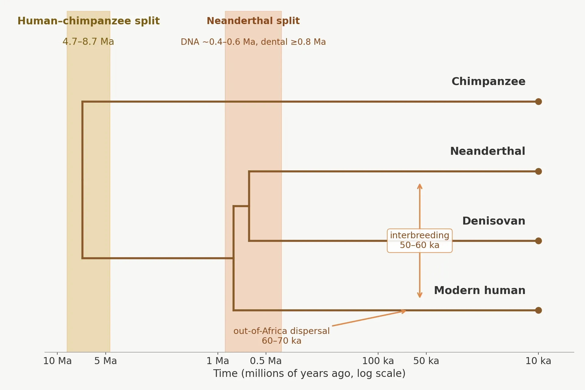
13. Dating Deep Time: The Tree of Life and the Cambrian Debate
Take the molecular clock to its deepest uses and the stakes rise. The origin of animals, the origin of placental mammals, the origin of life itself: these are the dates that shape our picture of the history of life, and they are the dates where the clock and the fossil record most often disagree. The disagreements are not a sign that one side is wrong. They are a sign that deep time is hard, that calibrations are scarce, that saturation erodes the signal, and that rate variation compounds with depth. The honest response is to report the ranges, explain the models, and show where the field is converging.
13.1 LUCA: ~4.2 billion years ago
LUCA, the last universal common ancestor, the single population from which all living things descend, is dated by the molecular clock to about 4.2 billion years ago. Moody and colleagues, in 2024, used pre-LUCA gene duplications, calibrated with microbial fossils and isotope records, under a relaxed-clock model, to estimate LUCA at 4.09 to 4.33 billion years ago, with a 95 percent confidence interval under the independent-log-normal relaxed-clock model. The composite age range across models is 3.94 to 4.52 billion years. LUCA's inferred genome was at least 2.5 megabases, 2.49 to 2.99 megabases, encoding about 2,600 proteins. It was a prokaryote-grade anaerobic acetogen, living without oxygen, with an early immune system (Moody et al. 2024).
That date is extraordinary for two reasons. First, it puts LUCA close to the origin of the Earth itself, about 4.54 billion years ago, leaving only a few hundred million years for life to originate and diversify to the point where LUCA could exist. Second, it is dated not from fossils of LUCA, which do not exist, but from gene duplications that happened before LUCA, whose timing can be inferred from the molecular clock. The globin gene family is the classic example of dating by duplication: the duplication that produced haemoglobin and myoglobin predates the vertebrate radiation, and its date constrains the vertebrate tree. The method is the same one used for species splits, applied to genes instead. For the broader story of how life began, the Sciory article on The Origin of Life Explained: How Life Began on Earth covers the chemistry and the earliest evidence in full.
13.2 The origin of animals: 850–650 million years vs. fossils at 541
Molecular clocks put the origin of animals, the Metazoa, in the Tonian and Cryogenian periods, 850 to 650 million years ago, more than 100 million years before the first definitive animal fossils in the Cambrian, at about 541 million years ago (Cunningham et al. 2017). The gap looks alarming. It is smaller than it looks, for three reasons. First, fossils give minimum ages. The first fossil of an animal is not the first animal. It is the first animal that was abundant, widespread, and preservable enough to fossilise. The true origin is necessarily older. Second, the distinction between stem groups and crown groups matters. A molecular date for the origin of animals may date the stem lineage, the early branches that led to animals but were not yet recognisably animal, while the fossil record dates the crown group, the living phyla with preservable tissues. Third, modern relaxed-clock analyses do not predict crown representatives of most animal phyla in the Neoproterozoic. The molecular clock-fossil gap is smaller than often claimed, and it has narrowed as clocks have improved and fossils have accumulated.
The Cambrian base itself is dated to 541 million years ago, marked by the first appearance of the trace fossil Treptichnus pedum. By about 520 million years ago, virtually all animal phyla with preservable tissues are represented in the fossil record. The Sciory article on The Cambrian Explosion Explained: When Animal Life Took Off tells that story in full, and the molecular dates belong alongside it, not in opposition to it.
13.3 The placental mammal radiation: long fuse vs. explosive
The placental mammals present the same pattern at a smaller scale. Molecular dates for crown Placentalia, the group containing all living placental mammals and their common ancestor, cluster at about 92 to 101 million years ago. A 2023 timetree study gave 101.4 million years from DNA alignment, with a 95 percent highest posterior density interval of 94.6 to 108.2 million years, and 92.2 million years from protein alignment, with an interval of 85.1 to 99.8 million years (Liu et al. 2023). Undoubted crown placental fossils, by contrast, appear only after the Cretaceous-Palaeogene boundary at 66 million years ago, the asteroid impact that ended the dinosaurs. The gap is 25 to 35 million years, and it has generated three competing models.
The explosive model says all placental splits happened after 66 million years ago, in the empty ecological space left by the dinosaurs. The long-fuse model says the crown group originated 105 to 120 million years ago, and the splits happened gradually through the Cretaceous. The soft-explosive model (Phillips and Fruciano 2018) places the interordinal diversification spike at about 75–85 million years ago — a few Cretaceous placental lineages seeding a rapid radiation after the boundary — while the deepest superordinal splits are older, around 90–110 million years in most studies. It is an influential middle position, but it is still contested, and it is not a settled consensus. The fossil case against a deep Cretaceous radiation is strong: thousands of non-placental Cretaceous fossils are known, yet no undoubted crown placentals, as O'Leary and colleagues argued in 2013. The molecular case for a pre-boundary origin is also strong: the genetic distances are too large to fit into the post-boundary window without invoking implausibly fast rates. The soft-explosive model splits the difference, and it is where much of the field is converging, though the model remains contested. The Sciory article on Mass Extinctions Explained: The Big Five and the Sixth covers the K-Pg boundary and its aftermath in full.
13.4 Why deep dates carry the widest error bars
Deep dates are uncertain for reasons that compound. Calibrations are scarce: there are fewer fossils the deeper you go, and the ones that exist are harder to place on the tree. Saturation erodes the signal: fast genes have rolled over, and even slow genes are approaching their limit. Rate variation compounds: a rate shift early in the tree propagates through every date below it. The result is that a date for LUCA carries an error bar measured in hundreds of millions of years, while a date for the human-chimp split carries an error bar measured in millions. That is not a flaw in the method. It is the method reporting its own limits honestly. A date without error bars is a red flag at any depth. At deep time, it is a disqualification.
LUCA: about 4.2 billion years ago, 4.09–4.33 billion years under the relaxed-clock model, composite range 3.94–4.52 billion years.
Origin of animals: 850–650 million years by molecular clocks, versus first definitive fossils at 541 million years.
Crown placental mammals: about 92–101 million years by molecular clocks, versus undoubted crown fossils only after 66 million years.
No single number: every deep date is a range, and the range is the information.
14. Clocks on Fast-Forward: Viruses, Epidemics and Forensics
Now reverse the timescale. The same mathematics that dates LUCA at 4.2 billion years also dates a virus that emerged in November 2019. Viral genomes mutate so fast that the molecular clock ticks in weeks and months, not millions of years, and the dates it gives are precise enough to guide public health. This is the molecular clock at the other end of its range, and it is where the method becomes a tool for the present, not just a window on the deep past.
14.1 HIV: tracing a pandemic to Kinshasa, ~1920
HIV-1 group M, the lineage responsible for more than 95 percent of global HIV infections, originated from SIVcpz, the simian immunodeficiency virus of central African chimpanzees, with the key transfer happening in southeastern Cameroon and the virus spreading via the Sangha river to Kinshasa, then called Léopoldville (Faria et al. 2014; MDPI review 2025). The molecular clock dates the most recent common ancestor of group M to the early twentieth century. Worobey and colleagues, in 2008, used a 1960 lymph-node sample and the 1959 ZR59 sample, which were already about 12 percent divergent from each other, to date the viral ancestor to 1884 to 1924 (Worobey et al. 2008). Faria and colleagues, in 2014, placed the Kinshasa emergence at about 1920, with spread along colonial railways (Faria et al. 2014). The two studies agree: the pandemic began in a single city, in the early twentieth century, decades before AIDS was recognised as a disease in the 1980s. The virus was circulating, diversifying, and spreading along transport networks while medicine had no name for it. That is a sobering fact, and it is a fact the molecular clock established. The Sciory article on Virus Evolution Explained: How Viruses Mutate and Adapt covers the broader story of how viruses evolve and adapt.
14.2 SARS-CoV-2: dating an outbreak to weeks
SARS-CoV-2 is among the most precisely dated evolutionary events ever studied, because the samples are dated to the day. Each genome in the analysis carries a collection date, and those dates calibrate the molecular clock directly, by tip dating. Nie and colleagues, in 2020, estimated the time to the most recent common ancestor at 12 November 2019, with a 95 percent Bayesian credibility interval of 11 October to 9 December 2019, and an evolutionary rate of 9.90 × 10⁻⁴ substitutions per site per year, with an interval of 6.29 × 10⁻⁴ to 1.35 × 10⁻³, using Bayesian tip dating with an uncorrelated lognormal relaxed clock on 112 early genomes (Nie et al. 2020). An independent estimate by Liu and colleagues, from 12,909 genomes, gave a mutation rate of 8.69 × 10⁻⁴ per site per year and a time to the most recent common ancestor of 28 November 2019, with a 95 percent confidence interval of 20 October to 9 December 2019 (Liu et al. 2020). The two studies, using different datasets and methods, converge on the same window: late October to early December 2019, with a central estimate in mid to late November. Later work refined the picture: Pekar and colleagues (2022) found evidence for at least two separate introductions of the virus into humans (lineages A and B), with the first around mid-November 2019 — consistent with the November 2019 window above, but showing the origin was not a single event. That convergence, on a timescale of weeks, shows how far the method has come since Sarich and Wilson counted antibody reactions in 1967.
14.3 Influenza: the clock that never stops
Influenza A(H3N2) evolves at a rate that makes the human clock look frozen. Fitch and colleagues, in 1997, estimated that the HA1 domain of the haemagglutinin gene evolves at about 5.7 × 10⁻³ substitutions per site per year, or 5.7 nucleotide substitutions per year across the HA1 domain, based on 254 genes sampled from 1984 to 1996 (Fitch et al. 1997). The NS gene evolves at about 2 × 10⁻³ substitutions per site per year, about a million times the evolutionary rate of mammalian germline genes (Buonagurio et al. 1986). That speed is why flu vaccines must be remade every year. The virus outruns immunity by mutating, and the molecular clock measures that outrunning in real time. The same speed is what makes influenza a superb system for studying molecular evolution in action: you can watch the molecular clock tick, year by year, in a way you cannot watch it tick in mammals.
14.4 Dogs: domestication's moving date
Dogs present a different kind of dating problem: a domestication, not a speciation, and a date that has moved as the data have improved. Mitochondrial DNA divergence estimates for the dog and wolf split range from 5,400 to more than 100,000 years, a range so wide it is almost useless. Whole-genome studies narrow it to 13,000 to 32,000 years. Archaeological dog-like remains more than 30,000 years old are likely extinct lineages, not the ancestors of living dogs. The honest range for domestication is about 15,000 to 30,000 years (Parker and Gilbert 2015).
Ancient DNA sharpened the picture. A 35,000-year-old Taimyr wolf genome showed that the dog mutation rate was slower than assumed, placing the split between dog ancestors and present-day wolves before the Last Glacial Maximum, at least 27,000 years ago (Skoglund et al. 2015). That is the same pattern we have seen throughout this article: a new calibration, a slower rate, an older date. The dog story is not settled, and the range of 15,000 to 30,000 years is the honest summary. It is also a reminder that domestication is a process, not an event, and that the "date" of domestication depends on whether you mean the first wolf that lived alongside humans, the first population that was genetically distinct, or the first dog that looked like a dog.
14.5 Forensics and conservation
The fast clock has uses beyond pandemics. In forensics, the molecular clock can date a poaching event, trace the origin of a seized animal product, or establish whether two samples of ivory came from the same population. In outbreak tracing, it can reconstruct who infected whom, and when, by comparing the genomes of pathogens sampled from different patients. In conservation, it can date a population bottleneck, a fragmentation event, or an invasive species' arrival, by measuring the genetic distance between the invaders and their source population and dividing by a calibrated rate. These applications are brief here because they are young, and because each one deserves a fuller treatment than this article can give. The principle is the same in every case: differences accumulate with time, and a calibrated rate turns differences into dates. The timescale changes. The logic does not. These are plausible applications of the same principle, not established case results, and each one is still being validated in practice.
Virus | Rate (substitutions / site / year) | Time to most recent common ancestor |
|---|---|---|
HIV-1 group M | Not a single rate; dated by archival samples | Early 20th century; about 1920 in Kinshasa (range 1884–1924) |
SARS-CoV-2 | 9.90 × 10⁻⁴ (Nie et al. 2020); 8.69 × 10⁻⁴ (Liu et al. 2020) | 12 November 2019 (95% interval 11 Oct–9 Dec 2019); independent estimate 28 November 2019 |
Influenza A(H3N2) HA1 | About 5.7 × 10⁻³ | Ongoing; new variants emerge yearly, requiring annual vaccine updates |
Influenza A NS gene | About 2 × 10⁻³ | Ongoing; about a million times the mammalian germline rate |
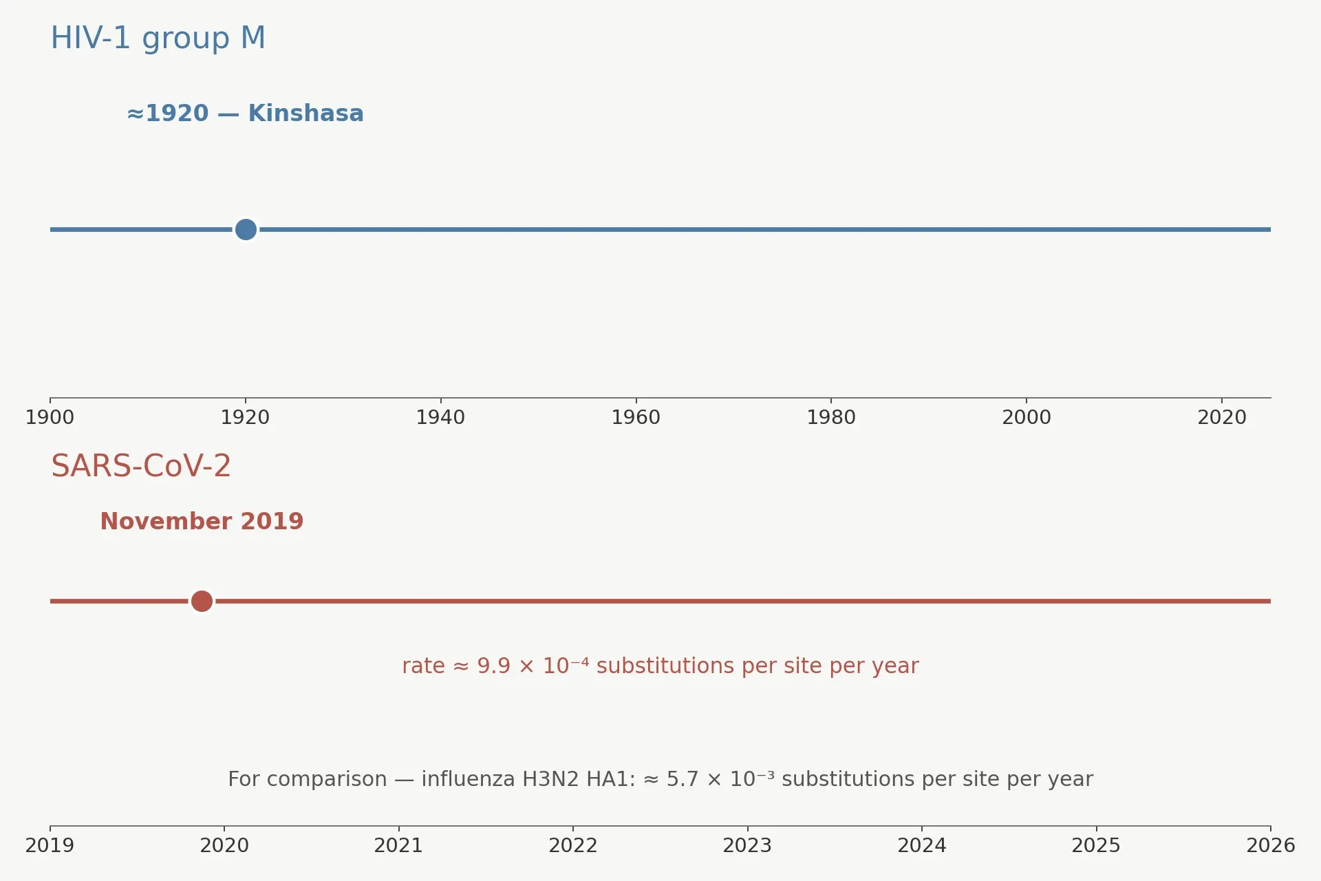
15. The Clock at Work Beyond Dating Splits
Dating species splits is the molecular clock's most famous job, but it is not its only one. The same mathematics dates populations, migrations, and gene families. The molecular clock is a general tool for putting time on genetic differences, and its applications extend well beyond the species tree.
15.1 Dating populations, not just species
Coalescence is the population-level version of the molecular clock. Take a gene variant carried by living people, trace its ancestry back through the generations, and ask when all copies of that variant last shared a common ancestor. That date is the coalescence time, and it is estimated the same way a species split is estimated: count the differences among the copies, divide by the rate. Human population splits, the divergence between African and non-African populations, the expansion into the Americas, the peopling of the Pacific, have all been dated this way, and the dates complement the archaeological record. A gene variant that is common in one population and rare in another carries a history, and the molecular clock reads it.
15.2 Biogeography: when continents and islands split lineages
Vicariance is the splitting of a population by a geological event: a continent breaking apart, a sea flooding a land bridge, a mountain range rising. The genetic distance between the populations on either side, divided by a calibrated rate, dates the vicariance event, and that date can be compared with the geological date for the same event. When the two agree, both are strengthened. When they disagree, one of them needs rethinking. Island colonisation is the mirror image: a single colonisation event, followed by radiation in isolation, dated by the genetic distances among the island species. The Sciory article on Animal Migration Explained: Why Animals Make Epic Journeys covers dispersal in the present, and the molecular clock extends that story into the past, dating the journeys that left no fossils.
15.3 Gene-family birthdays
Genes themselves have birthdays. A gene family, such as the globin family that includes haemoglobin and myoglobin, arises by duplication: a gene is copied, the copy diverges, and over time the two copies take on different functions. The duplication event can be dated by the genetic distance between the two copies, divided by the rate, in exactly the same way a species split is dated. Pre-LUCA duplications, the ancient duplications that happened before the last universal common ancestor, were the key to dating LUCA itself in §13.1. The molecular clock dates genes as readily as it dates species, because a duplication is a split, and a split is what the clock measures.
The connection to coevolution is worth a brief note. Gene families do not evolve in isolation. They evolve in the context of other genes, other species, and changing environments, and the timing of duplications can reveal when a new function arose in response to a new challenge. The Sciory article on Coevolution Explained: How Species Shape Each Other's Evolution explores that interplay in full.
15.4 Conservation genetics
Conservation genetics uses the molecular clock to date bottlenecks and fragmentation. A population that crashed to a handful of individuals, then recovered, carries a signature in its DNA: reduced diversity, and a coalescence time that clusters around the bottleneck. A population that was fragmented by habitat loss carries a different signature: genetic distances between fragments that grow with the time since fragmentation. Those dates help conservationists decide what to protect and how urgently. A population that has been isolated for ten thousand years is a different conservation priority from one that was isolated a century ago by a road. The molecular clock provides the timescale, and the timescale informs the decision. The Sciory article on Genetic Drift Explained: Bottlenecks and Founder Effects explains the drift side of the story, and the molecular clock adds the dates.
16. When the Clock and the Fossils Disagree
Disagreements between molecules and fossils are not failures. They are the moments when science learns something. A disagreement means one of the lines of evidence has been misread, or both have, or the two are dating different things and the gap is expected. The history of the molecular clock is, in large part, a history of such disagreements and their resolutions. Four cases tell the story.
16.1 Case 1: humans and apes (1967)
The original case, told in full in §1, ended in favour of the molecules. The fossil reading that put the human-ape split at 15 to 30 million years ago rested on Ramapithecus, and Ramapithecus turned out to belong on the orangutan line. The molecules, at about 5 million years, were right, and the fossils, reinterpreted, agreed. The lesson is not that molecules beat fossils. It is that a single fossil, read one way, can mislead a field, and that an independent line of evidence is the best protection against that kind of error. The Sciory article on the fossil record explains why fossil interpretations change as new specimens are found.
16.2 Case 2: the origin of animals
The animal-origins gap, 850 to 650 million years by molecules versus 541 million years by fossils, has narrowed but not closed. Early clock studies used poorly justified single calibrations and gave dates consistently too old. Modern relaxed clocks, with multiple calibrations and better models, agree better with the fossil record, but a gap remains. Part of the gap is expected: fossils give minimum ages, molecular dates give genetic isolation times, and the stem-group versus crown-group distinction accounts for some of the difference. Part of the gap may reflect a real phenomenon: early animals that were small, soft-bodied, and unlikely to fossilise. The gap is a research problem, not a verdict, and it is being worked on from both sides.
16.3 Case 3: placental mammals
The placental case, told in §13.3, is converging on a middle ground. The explosive model, all splits after 66 million years, and the long-fuse model, crown group at 105 to 120 million years, have both given way to the soft-explosive model: the interordinal diversification spike at about 75–85 million years ago, with the deepest superordinal splits older, around 90–110 million years, and the ordinal radiation after the boundary. It is an influential middle position, but the debate is not settled. That convergence is a model of how science resolves a disagreement: not by one side winning, but by a third position emerging that accommodates the strongest evidence from both sides. The molecular dates pushed the origin earlier than the fossils alone would suggest. The fossil absence pushed it later than the earliest molecular dates suggested. The middle ground is where the evidence points.
16.4 Case 4: Neanderthal split — molecules vs. teeth
The Neanderthal case is the one that remains unresolved, and it deserves to be stated plainly. DNA-based estimates put the modern human and Neanderthal population split at about 400,000 to 600,000 years ago. Dental evidence, from the rate of dental evolution in the Sima de los Huesos hominins, puts it at least 800,000 years ago. Those ranges do not overlap. One of them is wrong, or both are measuring different things, or the model that connects dental change to time is miscalibrated. As of 2026, the field has not settled the question, and this article will not pretend otherwise. An unresolved disagreement is not a failure of the method. It is a sign that the method is being used honestly, and that the next decade of work has a clear target.
16.5 Why disagreements happen (the checklist)
Disagreements have causes, and the causes are checkable. A bad calibration, a fossil misidentified or misdated, will bias every date that depends on it. A wrong rate, borrowed from a distant relative, will bias dates in one direction. Saturation will make deep dates too young. A gene tree that differs from the species tree, because of incomplete lineage sorting, where different genes trace different histories through a rapid radiation, or because of hybridisation and introgression, where genes move between species after they split, will mislead a single-gene clock. Neanderthal gene flow into modern humans is the classic example of the last problem: a gene that moved between species after the split will give a date that is too young for the split itself.
Is the calibration sound? Check the fossil identification, the fossil date, and whether the fossil gives a minimum age or has been treated as the split age.
Is the rate appropriate? Check whether it was measured in the same group, at a similar timescale, and whether it accounts for generation time and lineage variation.
Is saturation a factor? Check whether the gene is fast enough to have rolled over at this depth, and whether a correction model was applied.
Is the gene tree the species tree? Check whether incomplete lineage sorting or hybridisation could make a single gene misleading, and whether multiple genes agree.
Are the two methods dating the same thing? Check whether the molecular date is a genetic isolation time and the fossil date is a first-appearance date, in which case a gap is expected.
17. Myths and Misconceptions
Eight wrong ideas about the molecular clock circulate widely, in classrooms, in popular writing, and online. Each one has a short correction, and each correction has a reason. I disagree, directly and in my own voice, with the most common of them: the idea that the molecular clock is a single, steady timepiece. Most people assume the clock is one instrument, ticking at one rate, like a wristwatch. What the data actually show is a workshop full of instruments, each ticking at its own speed, each with its own range, each needing its own calibration. That is not a weakness. It is the reality of a method built from biology, and pretending otherwise is what produces the confident, wrong dates that later have to be corrected.
17.1 "The molecular clock ticks at a constant rate."
No. Rates vary by gene, by lineage, and over time within a lineage. Relaxed clocks exist because of this variation, and they are the standard tool for modern dating. A constant rate is a useful approximation for a narrow question, not a law of nature.
17.2 "There is one molecular clock."
No. Every gene is a different clock. There is no universal molecular clock, and not even a single molecular clock exists for a single organism. A mammal carries a mitochondrial clock, a nuclear clock, and a separate clock in every gene, each ticking at its own speed.
17.3 "DNA similarity percentages are exact."
No. "98 percent identical" depends on what you count. Single-letter differences alone give one figure. Insertions, deletions, and structural rearrangements give another. The method must be stated with the percentage, or the percentage is meaningless.
17.4 "The clock gives exact dates."
No. Every date is an estimate with a confidence or credibility interval. A date without error bars is a red flag. The precision limit is real: as one review of the field puts it, "the molecular clock cannot provide high levels of precision, but when used correctly it can still prove accurate: the lack of precision reasonably reflects our uncertainty about the past" (Gizmodo / The Conversation).
17.5 "Fossils and molecules are rival evidence."
No. The molecular clock needs fossils for calibration. Without fossils, it gives only relative time. Molecules and fossils are partners, and the best dates come from using both. The history of the field is a history of the two lines of evidence correcting each other.
17.6 "The molecular clock proves evolution."
No. The molecular clock is a tool that assumes common ancestry and measures timing within that framework. It does not prove common ancestry. The evidence for evolution is the consilience of independent lines: fossils, anatomy, embryology, biogeography, and genetics, all pointing the same way. The molecular clock contributes timing to that picture. It does not create the picture.
17.7 "A faster clock means faster evolution."
No. Molecular rate and morphological change are decoupled. A lineage can evolve rapidly in anatomy while its molecules tick slowly, and vice versa. Living fossils often have slow clocks, as §10.1 explains, because their lives run slow — but not always: some lineages with barely-changed bodies carry clocks that tick at ordinary speeds, or even fast. Rapid radiations, bursts of speciation, can happen with slow molecular clocks. Time and change are related, but they are not the same thing.
17.8 "The molecular clock is the same as the body clock / epigenetic clock."
No. Three different things share similar names. The evolutionary molecular clock dates species splits by counting DNA differences that accumulate over millions of years. The circadian clock is a 24-hour rhythm in gene expression that governs sleep and metabolism within a single lifetime. The epigenetic clock estimates age within an individual's lifetime from DNA methylation patterns. Each is a real concept. None is the other. The Sciory article on Epigenetics Explained: How Your Environment Changes Your Genes covers the epigenetic clock in its own context.
Constant rate? No — rates vary; relaxed clocks model the variation.
One clock? No — every gene is a different clock.
Exact percentages? No — the method must be stated with the number.
Exact dates? No — every date carries an interval.
Rivals? No — fossils calibrate the clock; they are partners.
Proof of evolution? No — the clock assumes common ancestry and measures timing within it.
Faster clock, faster evolution? No — molecular and morphological rates are decoupled.
Same as the body clock? No — evolutionary, circadian, and epigenetic clocks are three different things.
Convergence can also mislead the molecular clock, and it deserves a line of its own. Independently evolved similarities can be mistaken for close relatedness, as Al Tanner notes: "Evolution can be convergent, where different species independently evolve to appear similar, making it easy to mistake them for being closely related" (Gizmodo / The Conversation). The Sciory article on Convergent Evolution Explained: When Unrelated Species Look Alike covers convergence in full, and the warning applies to molecular dating as much as to anatomy.
18. What the Molecular Clock Cannot Do
A tool earns trust by stating its limits. This section is the one that earns this article its credibility, because it says plainly what the molecular clock cannot do, even when the rest of the article has shown what it can.
18.1 No calibration, no absolute dates
Without calibration, the molecular clock gives only relative time. A clock without a fossil anchor floats. It can say that one split is twice as old as another, but it cannot say how old either one is in years. Every absolute date in this article rests on a calibration, and every calibration rests on a fossil, a geological event, or a directly dated sample. Remove the calibrations and the dates vanish, leaving only the shape of the tree. That shape is valuable, but it is not a chronology.
18.2 Recent events are hard
Few mutations accumulate in centuries, and the ones that do are noisy. A split that happened a thousand years ago may have left no detectable differences in a slow gene, and a handful of differences in a fast one, with a wide uncertainty around the count. Time-dependency makes the problem worse. Ho and colleagues, in 2005, showed that short-term rates, under 1 to 2 million years, look much faster than long-term substitution rates, following a vertically translated exponential decay curve, with purifying selection as the most convincing explanation. The consequence, in their words, is that "it is invalid to extrapolate molecular rates of change across different evolutionary timescales" (Ho et al. 2005). Their phylogenetic mitochondrial DNA rates were about 0.5 percent per million years for birds, protein-coding, and about 1.5 percent per million years for primates, protein-coding and D-loop. Human mitochondrial DNA time-dependency has been confirmed with ancient genomes: observed rates range from 4.33 × 10⁻⁸ mutations per site per year in the most recent period to 1.91 × 10⁻⁸ in the oldest period, about 40,000 years ago, a 2.27-fold difference (Cabrera 2021). Apply a long-term rate to a recent event and you will date it too old. Apply a short-term rate to a deep event and you will date it too young. The rate must match the timescale.
18.3 Deep events are hard, for the opposite reason
Saturation erases signal at depth, as §11 explained. A fast gene that has rolled over many times carries no usable information about a split a billion years ago. A slow gene carries some, but with wide error bars. The deep-time wall is real, and it is why dates for LUCA carry error bars measured in hundreds of millions of years. The molecular clock can reach deep time. It cannot reach it precisely.
18.4 Gene trees are not species trees
A single gene can mislead, because the history of a gene is not always the history of the species that carry it. Incomplete lineage sorting happens when a rapid radiation leaves different genes with different histories: one gene says species A and B are closest, another says A and C are. Hybridisation and introgression move genes between species after they have split, so a gene that crossed from Neanderthals into modern humans will give a date for the gene flow, not for the species split. A single-gene clock is vulnerable to both problems. A multi-gene clock, which averages across many genes with different histories, is more robust, and it is the standard for that reason.
18.5 The clock cannot date a fossil, only a split
The molecular date is the genetic isolation time, the moment two populations stopped exchanging genes. That moment is always older than the first fossil of either descendant group, because a population must become distinct, then abundant, then fossilised, then found. A molecular date that is older than the first fossil is not a conflict. It is the expected pattern. A molecular date that is younger than the first fossil, by contrast, is a problem, because it implies the split happened after the fossil already existed. That check, simple as it sounds, catches real errors.
18.6 It cannot tell you WHY a lineage changed
Timing is not mechanism. The molecular clock can tell you when a lineage split, when a gene duplicated, when a virus emerged. It cannot tell you why the lineage split, what drove the duplication, or what made the virus spread. Those questions belong to ecology, to natural selection, to geology, and to history. The molecular clock dates. It does not explain adaptation, and anyone who uses a molecular date as an explanation for why something evolved has mistaken a timestamp for a cause.
19. Frequently Asked Questions (FAQ)
What is a molecular clock?
A molecular clock is a method for estimating when two species, populations, or genes last shared a common ancestor, by counting the genetic differences between them and applying the rate at which differences accumulate. DNA and protein sequences change at a roughly steady rate over time, so the number of differences between two species is proportional to the time since they split. The clock is statistical, not mechanical: its ticks are random mutations, and the count only becomes reliable when averaged over many sites and long times. It is used to date splits that fossils cannot reach, from the origin of animals hundreds of millions of years ago to the emergence of a virus a few years ago. The key idea is simple: more differences mean more time, and a calibrated rate turns differences into dates.
How do scientists use DNA to date evolution?
Scientists follow four steps. First, they pick the right gene for the depth of the question: fast genes for recent splits, slow genes for deep ones. Second, they align the gene sequences from the species being compared and count the differences, correcting for multiple hits at the same site. Third, they apply a substitution rate to turn the corrected distance into a date, using the equation time equals genetic distance divided by twice the rate, and they report the date with error bars. Fourth, they calibrate the rate with fossils, geological events, or directly dated ancient genomes, and they cross-check with a second gene and a second method. No serious date rests on a single gene. The method is described in full in §6, and the calibration step, which turns relative time into absolute dates, is the subject of §7.
What is the neutral theory?
The neutral theory, proposed by Motoo Kimura in 1968 and independently by Jack King and Thomas Jukes in 1969, states that most molecular change is selectively neutral: it does not affect the organism enough for natural selection to notice, and it accumulates by genetic drift at the mutation rate. The theory explains why the molecular clock can tick at a roughly steady rate: neutral mutations fix at the mutation rate, regardless of population size, so the substitution rate is set by chemistry, not by demography or by the environment. The theory applies only at the molecular level. It does not deny that natural selection shapes bodies, behaviours, and adaptations. It says that at the level of DNA letters, most change is neutral, and that neutral change is what the molecular clock measures. The nearly neutral theory, by Tomoko Ohta, refines the picture by allowing for slightly deleterious mutations whose fate depends on population size.
Who proposed the molecular clock?
Emile Zuckerkandl and Linus Pauling proposed the molecular clock in the early 1960s. In 1962 they noticed that amino-acid differences in haemoglobin lined up with fossil-based split times, and in 1965 they named the pattern the "evolutionary clock" and derived its mathematical form. Emanuel Margoliash, in 1963, provided the second founding observation: the equidistance of cytochrome c, in which a carp is equally distant from a frog, a turtle, a chicken, a rabbit, and a horse. Vincent Sarich and Allan Wilson, in 1967, provided the first dramatic application, dating the human-ape split to about 5 million years from blood proteins, against a fossil consensus of 15 to 30 million years. Motoo Kimura, in 1968, provided the mechanism, the neutral theory, that explained why the molecular clock could tick. The clock has many parents, and each one contributed a piece: the observation, the name, the application, and the theory.
Is the molecular clock accurate?
The molecular clock is accurate when used correctly, and misleading when used carelessly. Its accuracy depends on the calibration, the choice of gene, the correction for multiple hits, and the model used for rate variation. When those are done well, and when several genes and several calibrations agree, the dates are trustworthy, with error bars that honestly reflect the uncertainty. When they are done poorly, when a single gene is used, when a rate is borrowed from a distant relative, when a fossil age is treated as a split age, the dates can be badly wrong. The clock cannot deliver pinpoint precision, but when used correctly it can still prove accurate, and the width of its error bars honestly reflects our uncertainty about the past. The honest way to judge a molecular date is not to ask whether it is exact, but whether it carries error bars, whether it was cross-checked, and whether it agrees with independent evidence.
Why do different genes give different dates?
Different genes give different dates because they tick at different speeds, and because each gene has its own history. A fast gene, such as mitochondrial DNA in animals, accumulates differences quickly and is useful for recent splits, but it saturates at depth and gives dates that are too young for ancient splits. A slow gene, such as a highly conserved nuclear gene, accumulates differences slowly and is useful for deep splits, but it may show no differences at all for a recent split. Selection also matters: a gene under strong purifying selection ticks slower than a neutral gene, and a gene under positive selection ticks faster. Add to that the fact that different genes can have different histories, because of incomplete lineage sorting and hybridisation, and it is no surprise that single-gene dates disagree. The solution is to use several genes, understand why each one ticks at its speed, and report the range across genes, not a single number from one.
What is the difference between a molecular clock and a circadian clock?
The evolutionary molecular clock and the circadian clock share a name and nothing else. The evolutionary molecular clock estimates when two species split by counting the DNA differences between them and dividing by the rate at which differences accumulate. It measures time in mutations, and it never resets. The circadian clock is a molecular machine inside cells that runs a roughly 24-hour cycle, governing sleep, hormone release, and metabolism. It is built from a feedback loop in which CLOCK and BMAL1 proteins switch genes on and PER and CRY proteins switch them off again, once a day, and it resets every morning. The evolutionary clock answers the question: how many millions of years ago did two species split? The circadian clock answers the question: what time of day is it inside this cell? A third clock, the epigenetic clock, estimates age within a single lifetime from DNA methylation patterns. All three are real. None is the other.
The story that opened this article has not ended. Sarich and Wilson said about five million years. The modern range is about 4.7 to 8.7 million years, and the newest meta-analysis pushes the pooled estimate to about 7.3 to 8.7 million years. That drift is not a failure. It is the molecular clock getting sharper as genomes accumulate, as fossils are reinterpreted, and as models improve. The five-million-year "error" turned out to be right in the sense that mattered: the split was young, the old fossil reading was wrong, and a test tube could correct a museum. The exact number is still moving, and it will keep moving as new data arrive. That movement is what science looks like when it is working.
What the molecular clock has given us, in the end, is a dated tree of life. It runs from LUCA, about 4.2 billion years ago, through the origin of animals, 850 to 650 million years ago, through the placental radiation, through the human-chimp split, through the out-of-Africa dispersal 60,000 to 70,000 years ago, to a virus that emerged in November 2019. One method, one equation, one idea, that differences accumulate with time, spans that whole range. It is not a perfect timepiece. It is a statistical instrument, noisy at both ends, dependent on calibration, and honest about its uncertainty. Used with care, it is the best clock we have for the history of life, and it is still getting better.
Sources
Sarich, V. M. and Wilson, A. C. (1967). Immunological time scale for hominid evolution. Science 158(3805):1200–1203. PubMed
Wilson, A. C. and Sarich, V. M. (1969). A molecular time scale for human evolution. PNAS 63:1088–1093. PMC retrospective
UC Berkeley, Understanding Evolution. Sarich and Wilson and the human-ape split. Berkeley evolution site
Nature Education, Scitable. The Molecular Clock and Estimating Species Divergence. Nature Scitable
Penn State University (S. Blair Hedges). Probing Question: What is a molecular clock? Penn State
Astronoo. Molecular Clock: Time Inscribed in DNA. Astronoo
Circadian.news / Takahashi, J. S. (2017). The circadian clock genes and the molecular clock. Circadian.news
Ohno, M. (2019). Spontaneous de novo germline mutations in humans and mice: rates, spectra, causes and consequences. Genes & Genetic Systems 94(1):13–22. DOI
Kong, A. et al. (2012). Rate of de novo mutations and the importance of father's age to disease risk. Nature 488:471–475. Oxford summary
Campbell, C. D. et al. (2012). Estimating the human mutation rate using autozygosity in a founder population. Nature Genetics 44:1277–1281. PubMed
Zuckerkandl, E. and Pauling, L. (1962). Molecular disease, evolution, and genic heterogeneity. In Horizons in Biochemistry. Wikipedia, Molecular clock
Zuckerkandl, E. and Pauling, L. B. (1965). Evolutionary Divergence and Convergence in Proteins. In Evolving Genes and Proteins. PMC commentary
Margoliash, E. (1963). Primary Structure and Evolution of Cytochrome C. PNAS 50(4):672–679. DOI
Kimura, M. (1968). Evolutionary rate at the molecular level. Nature 217:624–626. DOI
Haldane, J. B. S. (1957). The cost of natural selection. Journal of Genetics 55:511–524. DOI
King, J. L. and Jukes, T. H. (1969). Non-Darwinian evolution. Science 164(3881):788–798. DOI
Ohta, T. (1973). Slightly deleterious mutant substitutions in evolution. Nature 246:96–98. DOI
Oxford Bibliographies. Neutral Theory. Oxford Bibliographies PDF
Wikipedia. Neutral theory of molecular evolution. Wikipedia
Cunningham, J. A. et al. (2017). The origin of animals: can molecular clocks and the fossil record be reconciled? BioEssays 39(1):1–12. DOI
Weir, J. T. and Schluter, D. (2008). Calibrating the avian molecular clock. Molecular Ecology 17:2321–2328. DOI
Brown, W. M., George, M. and Wilson, A. C. (1979). Rapid evolution of animal mitochondrial DNA. Proceedings of the National Academy of Sciences 76:1967–1971. DOI
Drummond, A. J. et al. (2006). Relaxed phylogenetics and dating with confidence. PLoS Biology 4:e88. DOI
Drummond, A. J. and Rambaut, A. (2007). BEAST: Bayesian evolutionary analysis by sampling trees. BMC Evolutionary Biology 7:214. DOI
Battistuzzi, F. U. et al. (2010). Performance of relaxed-clock methods in estimating evolutionary divergence times and their credibility intervals. Molecular Biology and Evolution 27:1289–1300. DOI
Heath, T. A., Huelsenbeck, J. P. and Stadler, T. (2014). The fossilized birth–death process for coherent calibration of divergence-time estimates. Proceedings of the National Academy of Sciences 111(29):E2957–E2966. DOI
Soares, P. and Rito, T. (2026). The evolution of molecular clocks: concepts, calibrations, and challenges. Biology 15(15):1329. DOI
Vawter, L. and Brown, W. M. (1986). Nuclear and mitochondrial DNA comparisons reveal extreme rate variation in the molecular clock. Science 234:194–196. DOI
Wolfe, K. H., Li, W.-H. and Sharp, P. M. (1987). Rates of nucleotide substitution vary greatly among plant mitochondrial, chloroplast, and nuclear DNAs. PNAS 84:9054–9058. DOI
Martin, A. P. and Palumbi, S. R. (1993). Body size, metabolic rate, generation time, and the molecular clock. Proceedings of the National Academy of Sciences 90:4087–4091. DOI
Martin, A. P. (1999). Substitution rates of organelle and nuclear genes in sharks: implicating metabolic rate (again). Molecular Biology and Evolution 16:996–1002. DOI
Nabholz, B. et al. (2008). Strong variations of mitochondrial mutation rate across mammals — the longevity hypothesis. Molecular Biology and Evolution 25(1):120–130. DOI
Stauffer, R. L. et al. (2001). Human and ape molecular clocks and constraints on paleontological hypotheses. Journal of Heredity 92:469–474. PubMed
Moorjani, P. et al. (2016). Variation in the molecular clock of primates. Proceedings of the National Academy of Sciences 113(38):10607–10612. DOI
Poszewiecka, B. et al. (2022). Revised time estimation of the ancestral human chromosome 2 fusion. BMC Genomics 23:616. DOI
Arnason, U. et al. (1998). Molecular timing of primate divergences as estimated by two nonprimate calibration points. Journal of Molecular Evolution 47:718–727. DOI
d'Oliveira Coelho, J. et al. (2026). Parting ways: Pan-Homo divergence revisited. Primates 67:549–565. DOI
Chimpanzee Sequencing and Analysis Consortium (2005). Initial sequence of the chimpanzee genome and comparison with the human genome. Nature 437:69–87. DOI
Britten, R. J. (2002). Divergence between samples of chimpanzee and human DNA sequences is 5%, counting indels. Proceedings of the National Academy of Sciences 99:13633–13635. DOI
Yoo, D. et al. (2025). Complete sequencing of ape genomes. Nature 641:401–418. DOI
Scally, A. and Durbin, R. (2012). Revising the human mutation rate: implications for understanding human evolution. Nature Reviews Genetics 13:745–753. DOI
Mendez, F. L. et al. (2016). The divergence of Neanderthal and modern human Y chromosomes. American Journal of Human Genetics 98:728–734. DOI
Meyer, M. et al. (2012). A high-coverage genome sequence from an archaic Denisovan individual. Science 338:222–226. DOI
Green, R. E. et al. (2010). A draft sequence of the Neandertal genome. Science 328:710–722. DOI
Reich, D. et al. (2010). Genetic history of an archaic hominin group from Denisova Cave in Siberia. Nature 468:1053–1060. DOI
Gómez-Robles, A. (2019). Dental morphological variation in the Sima de los Huesos hominins and the Neanderthal–modern human divergence. Science Advances 5(5):eaaw1268. DOI
Soares, P. et al. (2009). Correcting for purifying selection: an improved human mitochondrial molecular clock. American Journal of Human Genetics 84:740–759. DOI
Endicott, P., Ho, S. Y. W., Metspalu, M. and Stringer, C. (2009). Evaluating the mitochondrial timescale of human evolution. Trends in Ecology & Evolution 24:515–521. DOI
Moody, E. R. R. et al. (2024). The nature of the last universal common ancestor and its impact on the early Earth system. Nature Ecology and Evolution 8:1654–1666. DOI
Liu, G.-M. et al. (2023). Improved mammalian family phylogeny using gap-rare multiple sequence alignment: a timetree of extant placentals and marsupials. Zoological Research 44(6):1064–1079. DOI
O'Leary, M. A. et al. (2013). The placental mammal ancestor and the post–K-Pg radiation of placentals. Science 339:662–667. DOI
Phillips, M. J. and Fruciano, C. (2018). The soft explosive model of placental mammal evolution. BMC Evolutionary Biology 18:104. DOI
Nie, Q. et al. (2020). Phylogenetic and phylodynamic analyses of SARS-CoV-2. Virus Research 287:198098. DOI
Liu, Q. et al. (2020). Population genetics of SARS-CoV-2: disentangling effects of sampling bias and infection clusters. Genomics, Proteomics & Bioinformatics 18(6):640–647. DOI
Fitch, W. M. et al. (1997). Long-term trends in the evolution of H3 HA1 human influenza type A. PNAS 94:7712–7718. DOI
Buonagurio, D. A. et al. (1986). Evolution of human influenza A viruses over 50 years. Science 232:980–982. PubMed
Ho, S. Y. W. et al. (2005). Time dependency of molecular rate estimates and systematic overestimation of recent divergence times. Molecular Biology and Evolution 22:1561–1568. DOI
Cabrera, V. M. (2021). Human molecular evolutionary rate, time dependency and their impact on the mtDNA. Scientific Reports 11:5036. DOI
Gizmodo / The Conversation (Al Tanner, 2015). What Is the Molecular Clock, Exactly? Gizmodo
Alexiev, I. and Dimitrova, R. (2025). The origins and genetic diversity of HIV-1: evolutionary insights and global health perspectives. International Journal of Molecular Sciences 26(22):10909. DOI
Worobey, M. et al. (2008). Direct evidence of extensive diversity of HIV-1 in Kinshasa by 1960. Nature 455:661–664. DOI
Faria, N. R. et al. (2014). The early spread and epidemic ignition of HIV-1 in human populations. Science 346:56–61. DOI
Pekar, J. E. et al. (2022). The molecular epidemiology of multiple zoonotic origins of SARS-CoV-2. Science 377:960–966. DOI
Parker, H. G. and Gilbert, S. F. (2015). From caveman companion to medical innovator: genomic insights into the origin and evolution of domestic dogs. Advances in Genomics and Genetics 5:239–255. DOI
Skoglund, P. et al. (2015). Ancient wolf genome reveals an early divergence of domestic dog ancestors and admixture into high-latitude breeds. Current Biology 25(11):1515–1519. DOI
Nachman, M. W. and Crowell, S. L. (2000). Estimate of the mutation rate per nucleotide in humans. Genetics 156:297–304. DOI