
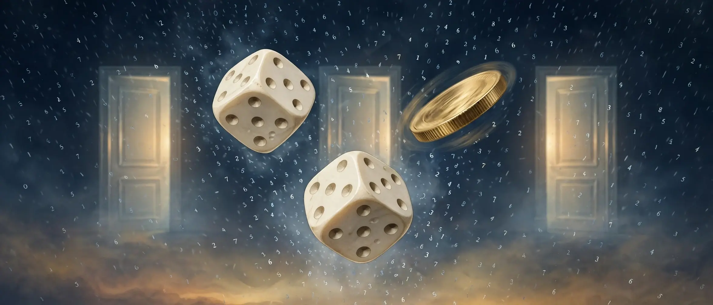
1. The Three Doors: A Puzzle That Fooled the Experts
Picture yourself on a television game show. In front of you stand three closed doors. Behind one of them is a car. Behind the other two are goats. You pick a door — say, door number one — and you do not open it yet. The host, who knows exactly where the car is, opens a different door, number three, and shows you a goat. Then he turns to you with the question that has embarrassed some of the cleverest people alive: do you want to stay with door one, or switch to door two?
Most people answer that it makes no difference. There are two doors left, one car and one goat, so the chance must be fifty-fifty, and switching is a coin toss. That answer feels like common sense. It is also wrong. If you switch, you win the car two times in three. If you stay, you win one time in three. Switching doubles your odds, and the reason is the whole subject of this article in miniature: information changes probability, and the host's action — the deliberate choice of which door to open — is information. To understand why, we need to answer the question this article is built around: what is probability, and how do you measure it?
I first met this puzzle as a student, and I gave the wrong answer with complete confidence. Fifty-fifty, I said, as if the arithmetic were obvious. A teacher asked me to play the game twenty times with three playing cards, switching every time, and count the wins. I won thirteen. Then I played twenty more times staying every time, and won seven. The numbers were not a proof, but they were a crack in my certainty, and through that crack the real mathematics came in. I have watched rooms full of clever adults make the same mistake since, including people who teach mathematics for a living. The puzzle is famous precisely because it separates what feels true from what is true, and that gap is where probability lives.
The puzzle is called the Monty Hall problem, after the host of the American game show Let's Make a Deal. It was first posed in print by the statistician Steve Selvin in 1975, and it became a national controversy in 1990 when Marilyn vos Savant published the correct answer — switch — in her Parade magazine column. She received thousands of letters telling her she was wrong, many of them from mathematicians with doctorates. She was not wrong. We will work the puzzle properly in section 8, with every case counted, and by the end of this article you will be able to explain to anyone, in two minutes, why switching wins two times in three.
But the three doors are only the hook. Probability is the mathematics of uncertainty, and uncertainty is everywhere: in the weather forecast on your phone, in the lottery ticket in your pocket, in the medical test result your doctor is explaining, in the insurance premium you pay every month, and in the spam filter that quietly sorts your email. This article is a plain-language guide to what probability is, how to calculate it, where intuition goes wrong, and how to use it without being fooled by it. We will start with the definition, walk through three hundred years of history, learn the handful of rules that generate the entire subject, and then put those rules to work on the two most famous puzzles in mathematics — the Monty Hall problem and the birthday paradox — before ending with the places probability quietly runs the modern world.
2. What Is Probability? A Number for "How Likely"
2.1 A number between zero and one
What is probability? It is a number that measures how likely something is. The number always sits between zero and one. Zero means the event cannot happen. One means it is certain. Everything else — every coin toss, every forecast, every lottery draw — lives somewhere in between, and the position on that scale is the whole content of the claim.
A fair coin landing heads has probability one half, written 0.5 or 50%. A fair die showing a six has probability one in six, about 0.167 or 16.7%. The sun rising tomorrow has probability so close to one that no one bothers to calculate it. A shuffled deck producing the same order of cards twice in a row has a probability so close to zero that it has effectively never happened in the history of card games. The scale is the same in every case, and that sameness is the point: probability gives us one language for talking about coin tosses, weather, disease, and spacecraft, because in every case we are answering the same question — how likely?
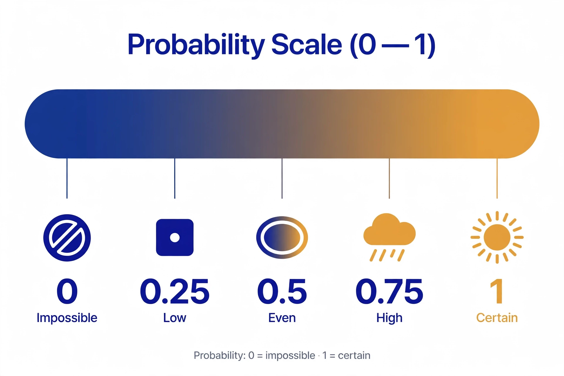
You can also write a probability as a percentage, as odds, or as "one chance in so many" — 50%, one half, evens, and one in two are four ways of saying the same thing. Scientists usually use the number between zero and one, because it makes the arithmetic clean. Bookmakers usually use odds, because they make the payout easy to see. We will translate between the two in section 13, and the translation is worth learning, because much of the confusion about probability in daily life comes from mixing up the two languages.
2.2 Three ways to think about it: classical, frequentist, subjective
There are three standard ways of thinking about what a probability means, and it helps to know all three, because different problems call for different lenses.
The classical view counts equally likely outcomes. A die has six faces, all equally likely, so the probability of a six is one favourable outcome divided by six total outcomes. This is the view we use for coins, dice, cards, and lotteries — anywhere the outcomes are symmetric by construction. It is the simplest view, and it is where we will do most of our calculating.
The frequentist view watches what happens over many repetitions. Flip a coin ten thousand times and the fraction of heads will be very close to one half — not exactly one half, but close, and closer the more you flip. On this view, a probability is a long-run frequency: the thing that the observed fraction settles towards as the number of trials grows. This is the view behind the law of large numbers, which we will meet in section 11, and behind every claim of the form "this drug works in 70% of patients", which means that out of a large group of similar patients, about seven in ten improved.
The subjective view treats probability as a degree of belief. When a weather forecaster says there is a 30% chance of rain tomorrow, she is not counting equally likely tomorrows and she has not watched ten thousand identical tomorrows. She is stating, as a number, how confident she is, given everything the models say. This is the view behind Bayes' theorem, which we will meet in section 7: probability as a measure of reasonable belief, updated as evidence arrives.
These three views are not rival theories fighting over the truth. They are three lenses for one idea, and working mathematicians switch between them without apology. The counting view tells you the probability of a six. The frequency view tells you what to expect over a long evening at the casino. The belief view tells you how to revise your mind when a test result comes back positive. What unites them is the arithmetic: whichever lens you use, the numbers must obey the same three rules, and those rules are the subject of section 4.
2.3 Why a single number is enough — and what it cannot do
A single number between zero and one seems like a thin thing to carry all of uncertainty. It is enough, though, because the number is not a description of the world — it is a description of our knowledge of the world. The coin is already in the air; the outcome is fixed by physics the moment it leaves the thumb. Probability does not claim to predict that outcome. It claims to summarise, exactly, what a reasonable person should expect given what they know.
That is also its limit, and the limit matters. Probability never tells you what will happen next. A 90% chance of rain does not promise rain, and a 10% chance does not promise dry weather. A lottery ticket with a 1-in-292-million chance can still win — someone's ticket does, eventually. Probability speaks about collections of similar situations, and about fair prices for gambles, and about how to change your mind when evidence arrives. It is silent about the single case in front of you, except to say how much you should be willing to bet on it. If you remember one sentence from this section, make it this one: what is probability? A number between zero and one that measures how likely something is, given what you know. Anyone who tells you otherwise is selling something, and section 12 is a catalogue of the ways that mistake is made.
3. A Very Short History: Dice, Letters, and a 300-Year Argument
3.1 The problem of points: Pascal and Fermat, 1654
Probability theory was born in a gambling dispute. The problem was called the problem of points, and it had been annoying mathematicians since Luca Pacioli wrote about it in his Summa de Arithmetica in 1494. Two players are playing a game of chance for a stake of money. The game is interrupted before anyone has won. How should the stake be divided fairly?
In 1654, a French nobleman and gambler, the Chevalier de Méré, put the problem to Blaise Pascal, who wrote to Pierre de Fermat for help. Their letters of that year are the founding documents of probability theory, and the solution they reached is worth working through, because it contains the whole idea of expected value in embryo.
Take a simple version. Two players are racing to five points, and the game is stopped with the score at four to three. The stake is 64 coins. What is each player's fair share? Pascal's reasoning goes like this. Play one more round. Half the time, the leading player wins it, reaches five points, and takes all 64 coins. Half the time, the trailing player wins it, the score is level at four each, and the last point is a coin toss — worth 32 coins on average. So the leading player's fair share is half of 64 plus half of 32, which is 48 coins, and the trailing player's share is 16.
The move that matters is the one Pascal and Fermat both made: stop asking who deserves the money, and start asking what would happen if the game continued. The fair division is the average of the possible futures, weighted by their probabilities. That idea — that a chance is worth the average of its outcomes — became expected value, and expected value became the engine of the whole subject. We will use it in section 10 to price lottery tickets and insurance policies, and the arithmetic will be exactly the same as it was in 1654.
3.2 Huygens writes the first textbook (1657) and Bernoulli's great book (1713)
Three years after the Pascal–Fermat letters, the Dutch scientist Christiaan Huygens published De Ratiociniis in Ludo Aleae — On Reasoning in Games of Chance — in 1657. It was the first printed textbook on probability, and it stayed the standard text for about fifty years. Huygens' great contribution was to make expected value formal: the value of a chance is the sum of each outcome multiplied by its probability. He proved it from a single principle — that a fair game is one in which each player's expected gain is zero — and built the subject up from there, proposition by proposition. The full text of his treatise, in an English translation, is available from Dartmouth's Huygens archive.
Meanwhile, Gerolamo Cardano had written Liber de Ludo Aleae, the Book on Games of Chance, in the 1500s, though it was only published after his death, in 1663. Cardano had worked out the counting of dice outcomes correctly, including the fact that some totals are more likely than others — the observation we will use in section 5 to explain why seven is the luckiest total on two dice.
The next great leap came from Jacob Bernoulli, whose Ars Conjectandi — The Art of Conjecturing — was published in 1713, eight years after his death, by his nephew Nicolaus. Bernoulli worked on the book's final part for about twenty years, and it contains the first law of large numbers: the theorem that observed frequencies close in on true probabilities as the number of trials grows. It is the result that connects the counting view of probability to the frequency view, and it is the reason a casino can be sure of its profits even though it cannot predict a single spin. We will meet it properly in section 11.
3.3 Bayes, Laplace, and the long road to rigour — Kolmogorov, 1933
The eighteenth century belonged to two men. Thomas Bayes, an English minister and mathematician, wrote an essay on how to work backwards — from an observed event to the probability of its cause — and it was read to the Royal Society in 1763, two years after his death, then published in the Philosophical Transactions in 1764. Pierre-Simon Laplace independently developed the same updating rule in 1774 and laid it out in full in his Théorie analytique des probabilités in 1812. The rule is now called Bayes' theorem, and it is the most useful single formula in the subject. It is also the most misunderstood, and section 7 is devoted to getting it right.
Abraham de Moivre, working in the 1730s, found that the distribution of coin-toss results settles into the bell curve — the normal distribution — as the number of tosses grows. Laplace extended the result, and it became the central limit theorem: the reason opinion polls can quote a margin of error, and the reason the bell curve shows up everywhere from heights to test scores. How calculus works sits behind some of this machinery — the bell curve is defined by an integral — but the probability ideas stand on their own, and we will use them without any calculus at all.
For all this progress, probability still lacked a foundation. What exactly is a probability, and what rules must it obey? The answer came in 1933, when the Russian mathematician Andrey Kolmogorov published a monograph of about sixty pages, Foundations of the Theory of Probability, that put the subject on three axioms. Probability became a branch of measure theory — the mathematics of assigning sizes to sets — and every formula in the subject became a logical consequence of those three rules. We meet them next.
4. The Rules of the Game: Sample Spaces and the Three Axioms
4.1 Sample spaces and events
Every probability problem starts by listing what can happen. The list is called the sample space, and each item on it is an outcome. An event is a collection of outcomes — a set we care about.
Flip a coin. The sample space is two outcomes: heads, tails. Roll a die. The sample space is six outcomes: one through six. Draw a card from a shuffled deck. The sample space is fifty-two outcomes. The event "roll an even number" is the set of outcomes two, four, and six — three outcomes out of six, so the probability is three in six, or one half.
Two dice give a bigger sample space: thirty-six pairs of numbers, from one-and-one to six-and-six. The event "the total is seven" is the set of six pairs — one-and-six, two-and-five, three-and-four, four-and-three, five-and-two, six-and-one — so the probability is six in thirty-six, or one in six. We will draw this grid in section 5, because seeing the thirty-six squares makes the counting obvious in a way that symbols never do.
The discipline of writing the sample space down before calculating anything is the single most useful habit in probability. Most errors in the subject — including the famous ones in section 12 — come from counting the wrong sample space, or from treating outcomes as equally likely when they are not. A coin that has landed heads five times in a row still has a sample space of two outcomes on the sixth toss, and the probability of heads is still one half. The wheel that has shown black twenty-six times in a row still has eighteen black pockets and eighteen red ones. The sample space does not remember.
4.2 Kolmogorov's three axioms, in plain words
Kolmogorov's axioms are three rules that any sensible assignment of probabilities must obey. They are short enough to state in a paragraph, and everything else in probability follows from them.
First, non-negativity: no event can have a negative probability. A probability is a size, and sizes are never negative.
Second, normalisation: the probability of the whole sample space is exactly one. Something must happen. The total probability of all possible outcomes is one, which is the same as saying 100%.
Third, additivity: if two events cannot happen at the same time — if they are mutually exclusive — then the probability that one or the other happens is the sum of their probabilities. The chance of rolling a one or a two on a die is one sixth plus one sixth, which is one third. For an infinite list of mutually exclusive events, the same rule holds: add them all up.
That is the whole foundation. It does not say what probability is — whether it is a frequency, a degree of belief, or a count of symmetric outcomes. It says what probability must do, and any rule that satisfies the three axioms is a probability. The three interpretations from section 2 are three different ways of producing numbers that obey these rules.
4.3 What follows from the axioms: the complement and addition rules
A surprising amount of the subject falls out of the three axioms with a few lines of arithmetic. The most used result is the complement rule: the probability that an event does not happen is one minus the probability that it does. P(not A) = 1 − P(A). It is often easier to calculate the chance that something fails than the chance that it succeeds, and the complement rule lets you flip the problem. The birthday paradox in section 9 is solved this way: instead of counting the chance that two people share a birthday, we count the chance that nobody does, and subtract from one.
The addition rule follows from the third axiom, with one correction. If two events can overlap — if both can happen at once — then adding their probabilities counts the overlap twice, so you must subtract it once: P(A or B) = P(A) + P(B) − P(A and B). Draw two cards and ask for the chance of a heart or a face card: thirteen hearts plus twelve face cards, minus the three face cards that are hearts, gives twenty-two out of fifty-two. Forget the subtraction and you get an answer that is too big, and the error is the kind that shows up in real arguments about risk, where people add up dangers as if they never overlapped.
The multiplication rule for independent events also follows, once independence is defined: if knowing that B happened tells you nothing about A, then P(A and B) = P(A) × P(B). Two coin tosses are independent, so the chance of two heads is one half times one half, one quarter. Two cards drawn without replacement are not independent, because the first draw changes the deck — and that dependence is the subject of section 6.
5. How to Calculate Probability: The Counting Method
5.1 Favourable over total — when it works
The workhorse formula of probability is the simplest one in the subject: when every outcome is equally likely, the probability of an event is the number of favourable outcomes divided by the total number of outcomes. That is all there is to it, and the difficulty is never the division. The difficulty is always the counting — making sure the favourable outcomes are counted once each, and making sure the total is the right total. It is the oldest answer to the question of what is probability in games of chance, and it still does most of the work in the subject.
A coin gives two outcomes, one favourable to heads, so the probability is one half. A die gives six outcomes, one favourable to a six, so the probability is one in six. A shuffled deck gives fifty-two outcomes, four favourable to an ace, so the probability is four in fifty-two, or one in thirteen. The formula is honest only when the outcomes really are equally likely, and that condition is doing all the work. A die with a weight inside it does not have six equally likely outcomes, and the formula does not apply. A deck that has not been shuffled does not have fifty-two equally likely cards. Probability begins with symmetry, and where there is no symmetry, you need a different method — usually the frequency view, watching what actually happens over many trials.
5.2 Two dice: why seven is the luckiest total
Two dice are the classic example, because they show how a simple counting problem can defeat intuition. Roll two fair dice and add the numbers. Which total is most likely? Many people guess that all totals are equally likely, or that the middle total must be seven "because it is in the middle" without being able to say why. The counting settles it.
There are thirty-six equally likely pairs: six results on the first die times six on the second. The total of two can happen only one way, one-and-one. The total of three can happen two ways, one-and-two and two-and-one. Four has three ways, five has four, six has five, and seven has six: one-and-six, two-and-five, three-and-four, four-and-three, five-and-two, six-and-one. Then the counts fall away again: eight has five ways, nine has four, ten has three, eleven has two, and twelve has one. The most likely total is seven, with probability six in thirty-six, or one in six. The least likely totals, two and twelve, each have probability one in thirty-six.
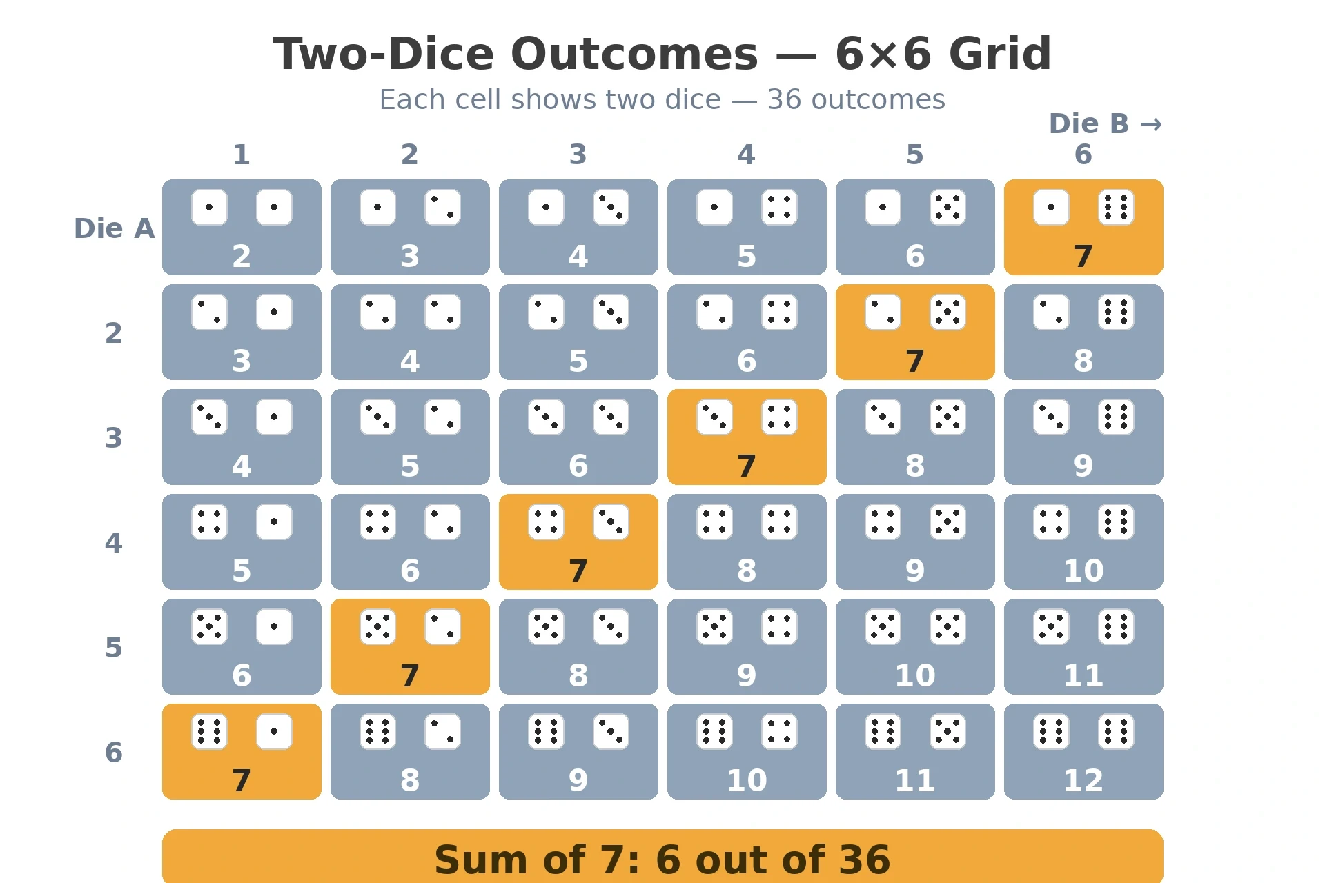
Cardano worked this out in the 1500s, and gamblers had known it in practice long before anyone wrote it down: the dice do not care what you want, and the totals in the middle simply have more ways to happen. The same counting idea scales up. Three dice have 216 outcomes. A poker hand has 2,598,960 possible five-card combinations. Every casino game, every lottery, and every card trick that claims to beat the odds is, at bottom, a counting problem — and the house employs people who can count.
5.3 Counting without listing: combinations and the Powerball
Listing thirty-six dice pairs is easy. Listing the combinations of a lottery is not, and that is where the mathematics of counting — combinatorics — earns its keep. The number of ways to choose five items from sixty-nine, order not mattering, is written C(69,5), and it equals 11,238,513. The Powerball game asks you to choose five white balls from sixty-nine, and then one red Powerball from twenty-six. Every choice of five white balls can sit alongside any of the twenty-six red balls, so the total number of possible plays is 11,238,513 times 26, which is 292,201,338. Your ticket holds exactly one of those combinations. Your chance of the jackpot is one in 292,201,338.
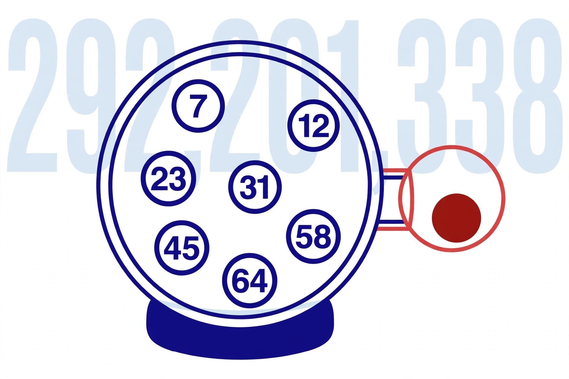
The odds of winning any prize are much friendlier — about one in 24.87 — because most prizes are small, and the most likely win is matching only the red ball, which happens about one time in thirty-eight. But the jackpot is the number that matters for the fantasy, and the fantasy is the product being sold. A play costs two dollars, and drawings happen three times a week, on Monday, Wednesday, and Saturday. If you bought one ticket for every drawing, you would expect to wait about 1.87 million years to hit the jackpot once. We will come back to what that means for the value of a ticket in section 10.
The counting method has a limit, and it is worth naming. It works when the outcomes are symmetric and you can count them. It does not work for the chance that it rains tomorrow, or that a patient recovers, or that a bridge stands for a century. Those probabilities come from models, from data, and from judgement — the frequency and belief views of section 2. The counting method is the cleanest room in the house, and most of life happens in the other rooms.
6. Conditional Probability: When New Information Changes the Answer
6.1 What "given that" means
Conditional probability is the probability of an event given that something else has happened. The words "given that" are the whole idea. The probability that a card is a king is four in fifty-two, one in thirteen. But the probability that a card is a king given that it is a face card is different: there are twelve face cards, and four of them are kings, so the probability is four in twelve, or one in three. The new information shrank the sample space from fifty-two cards to twelve, and the probability changed with it.
The formula is P(A given B) = P(A and B) divided by P(B). In words: among the cases where B happened, what fraction also had A happen? It is a simple idea, and it is the idea that the Monty Hall problem turns on — the host's opening of a goat door is new information, and it changes the probabilities, but only for the doors the host could have opened. It is also the idea behind Bayes' theorem, which is the next section, and behind every medical test, spam filter, and weather model in the modern world.
6.2 Independent vs dependent events
Two events are independent when knowing that one happened tells you nothing about the other. Two coin tosses are independent: the coin has no memory, and five heads in a row change nothing about the sixth toss. The probability of heads stays one half, and anyone who tells you that tails is "due" is making the mistake we will dissect in section 12.
Two cards drawn from a deck without replacement are dependent. Draw one card and it is an ace: the chance that the next card is an ace has fallen from four in fifty-two to three in fifty-one, because one ace is gone and the deck is smaller. Draw one card and it is not an ace, and the chance that the next is an ace has risen slightly, to four in fifty-one. Dependence is not mysterious; it is bookkeeping. The sample space changed, so the numbers changed.
Dependence is everywhere once you look for it. Rain today makes rain tomorrow more likely, because weather systems persist. A positive test result makes a disease more likely, because the test and the disease are linked. A student's score on one exam predicts their score on the next, because both measure the same preparation. Independence is the special case, not the rule — and assuming independence when events are dependent is one of the most expensive mistakes in applied statistics. It is, for example, how people underestimate the chance of two rare failures happening together in an engineered system, when both failures share a single cause.
6.3 The multiplication rule
For independent events, the probability that both happen is the product of their probabilities: P(A and B) = P(A) times P(B). Two heads in a row: one half times one half, one quarter. Three heads in a row: one eighth. Ten heads in a row: one in 1,024 — rare, but not impossible, and it will happen to someone, somewhere, every day, because a great many coins are tossed every day. Rarity is not impossibility, and a probability of one in a thousand means that in a thousand trials, it happens about once.
For dependent events, the multiplication rule needs the conditional probability: P(A and B) = P(A) times P(B given A). Two aces in a row from a shuffled deck: four in fifty-two times three in fifty-one, which is twelve in 2,652, or one in 221. The difference between the two versions of the rule is the difference between a coin and a deck of cards, and keeping them straight is the difference between a correct calculation and a confident error.
A tree diagram makes all of this visible. Draw a branch for the first event, split it into outcomes, then draw branches for the second event from each outcome, and multiply along the paths. The diagram for two coin tosses has four paths, each with probability one quarter. The diagram for two cards has paths with different probabilities, because the second branch depends on the first. If you ever find yourself confused by a probability problem, draw the tree. It is the cheapest thinking tool in the subject, and professional statisticians use it too.
7. Bayes' Theorem: How to Change Your Mind Correctly
7.1 The formula, in words
Bayes' theorem is a formula for updating a belief when new evidence arrives. In words: the probability of a hypothesis after seeing the evidence equals the probability of the evidence if the hypothesis were true, times the probability you gave the hypothesis before the evidence, divided by the total probability of seeing that evidence at all. Written with symbols, P(A given B) = P(B given A) times P(A), divided by P(B).
It looks like a piece of bookkeeping, and it is. But it is the bookkeeping that runs the world. Every spam filter, every medical screening programme, every weather model, and every machine-learning classifier is Bayes' theorem in disguise: start with a prior — what you believed before — multiply by how likely the evidence is under each hypothesis, and read off the updated odds. The theorem is named after Thomas Bayes, whose essay on the subject was read to the Royal Society in 1763 and published in the Philosophical Transactions in 1764, and it was developed into a general method by Pierre-Simon Laplace in 1774 and 1812. A full account of the theorem's history and proof is on Wikipedia's Bayes' theorem page.
The part people get wrong is the prior. Bayes' theorem does not let you ignore what you believed before the evidence arrived. It forces you to state it, as a number, and then it shows you exactly how much the evidence should move you. A strong piece of evidence moves a weak prior a long way. A weak piece of evidence barely moves a strong prior at all. And a test result that sounds decisive can be nearly worthless if the thing it tests for is rare enough — which brings us to the most famous example in the subject.
7.2 The disease-test example: why a 99% accurate test can be wrong 91% of the time
Suppose a disease affects one person in a thousand. A test for the disease is 99% accurate in both directions: 99% of sick people test positive, and 99% of healthy people test negative. You take the test, and it comes back positive. What is the chance you actually have the disease?
Most people answer 99%. The correct answer is about 9%. Here is the arithmetic, done slowly, because the surprise is in the counting.
Imagine a million people take the test. One in a thousand of them is sick, so about 1,000 people have the disease and 999,000 do not. Of the 1,000 sick people, 99% test positive: 990 true positives. Of the 999,000 healthy people, 1% test positive anyway: 9,990 false positives. So the total number of positive results is 990 plus 9,990, which is 10,980 — and only 990 of those belong to people who are actually sick. The chance that a positive result means the disease is 990 divided by 10,980, which is about 0.09, or 9%.
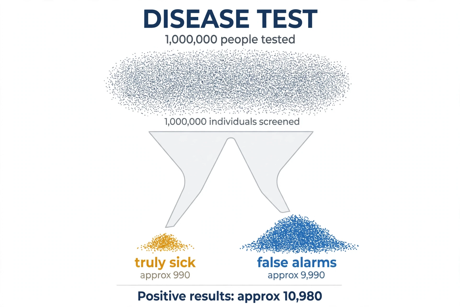
The test is not broken. It really is 99% accurate. The problem is the base rate: the disease is so rare that the healthy population is a thousand times bigger than the sick one, and even a 1% error rate in that huge group produces ten times as many false alarms as there are true cases. This is called base-rate neglect, and it is one of the most consequential reasoning errors in medicine, in law, and in everyday judgement. It is why screening programmes for rare diseases produce far more scares than diagnoses, and why a doctor who understands Bayes' theorem will order a second, different test before telling a patient anything definite. How vaccines work and how blood works both touch on screening and testing, and the same arithmetic applies there.
7.3 Base rates: the mistake almost everyone makes
Base-rate neglect is the habit of ignoring how common something is before the evidence arrived. It shows up far beyond medicine. A hiring manager who is impressed by a candidate's performance on a test that most applicants pass anyway has neglected the base rate. A jury that hears that a DNA match would occur by chance in one person in a million, and concludes that the chance the defendant is innocent is one in a million, has made the same error — the prosecutor's fallacy. The match statistic is P(evidence given innocence): the chance of seeing this DNA profile if a random person left the sample. What the jury needs is P(innocence given evidence): the chance that this defendant is innocent, given the match — and that depends on how many other people could also match, and on all the other evidence in the case. Confusing the two directions of a conditional probability is easy, because the sentences sound alike. The numbers are not alike at all.
Bayes' theorem is the cure, and the cure is a habit, not a formula. Before you update, ask: how common was this before I saw the evidence? A rare thing needs very strong evidence to become likely. A common thing needs only a nudge. Keep the base rate in view, and most of the famous paradoxes in this subject dissolve into arithmetic.
There is a deeper point here, and it is why Bayes' theorem has passionate defenders and equally passionate critics among statisticians. The theorem needs a prior — a number for what you believed before — and where that number comes from is a matter of judgement. Frequentists prefer methods that avoid priors altogether. Bayesians reply that everyone has a prior, whether they admit it or not, and that writing it down honestly is better than hiding it. For this article, the practical lesson is enough: when new evidence arrives, do not ask "how accurate is this test?" Ask "how accurate is this test, and how common is the thing it tests for?" The second question is the one that decides the answer.
8. The Monty Hall Problem, Worked Properly
8.1 The setup, stated precisely
We promised to come back to the three doors, so here they are, stated with the precision the puzzle needs. Three doors. Behind one is a car; behind the other two are goats. You pick a door — say door one — and you do not open it. The host, who knows where the car is, opens a different door — say door three — and shows you a goat. He always does this: he always opens a door you did not pick, he always shows a goat, and he always offers you the chance to switch. The question is: should you switch to door two, or stay with door one?
The precision matters, because the answer depends on it. If the host opened a door at random and happened to reveal a goat, the answer would be different — it would be fifty-fifty, and switching would gain nothing. But that is not the game. The host knows, he chooses, and his choice carries information. The whole puzzle is about what that information is worth.
8.2 Why switching wins two times in three
Count the cases. The car is equally likely to be behind any of the three doors, so there are three cases, each with probability one third.
Case one: the car is behind door one, the door you picked. The host can open either door two or door three, since both hide goats. If you switch, you lose. If you stay, you win.
Case two: the car is behind door two. The host must open door three — it is the only goat door he can open, since he cannot open your door and cannot open the car door. If you switch to door two, you win. If you stay, you lose.
Case three: the car is behind door three. The host must open door two. If you switch, you win. If you stay, you lose.
Switching wins in two of the three cases. Staying wins in one. The probability of winning by switching is two thirds; by staying, one third. That is the whole proof, and it fits in a paragraph — which is why the puzzle is so unsettling. Thousands of people, including professional mathematicians, read that proof in 1990 and refused to believe it.
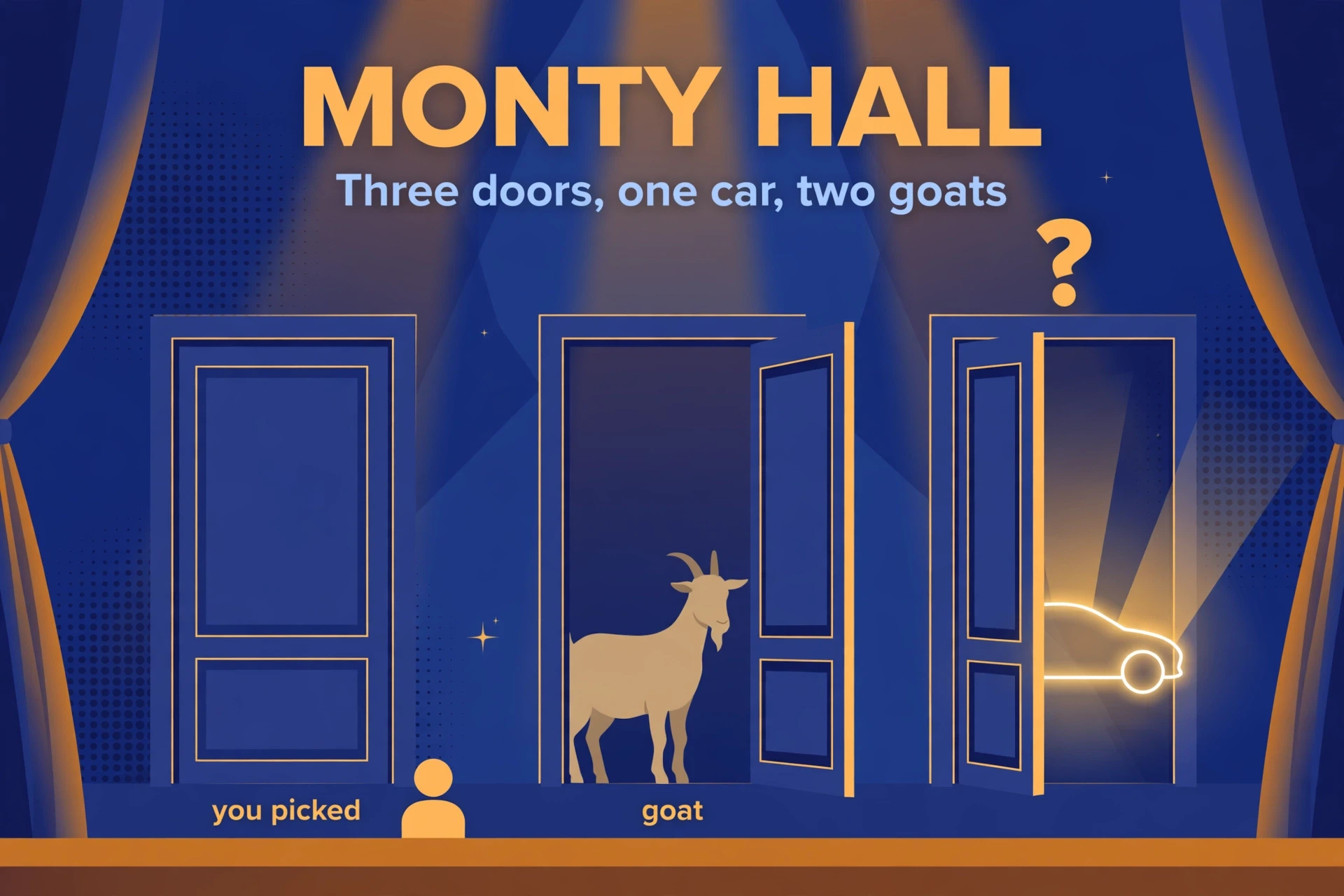
The intuitive error is to think that the host's action tells you nothing, because a goat was always going to be revealed somewhere. But the host's action tells you a great deal — it tells you which door he avoided. Your door keeps its original one-third chance, because nothing the host did touched it: he never opens your door, and he never gives you information about it. The other two doors shared two thirds between them, and when the host removes one of them, the whole two thirds concentrates on the door that remains. Switching captures that concentrated probability; staying throws it away.
8.3 The 100-door version that makes it obvious
If the three-door version still feels wrong, scale it up. Imagine one hundred doors. One hides a car; ninety-nine hide goats. You pick one door. The host, who knows where the car is, opens ninety-eight other doors, all showing goats, and offers you the one remaining closed door. Do you switch?
Now the answer feels obvious, and it should: your first pick had a one-in-a-hundred chance, and nothing has changed that. The other ninety-nine doors shared ninety-nine chances in a hundred, and the host has eliminated ninety-eight of them, leaving all ninety-nine chances concentrated on a single door. Switching wins ninety-nine times in a hundred. The three-door game is the same game with smaller numbers — the only difference is that with three doors, the concentration is less dramatic, and the wrong answer feels more plausible. The mathematics does not care how dramatic it feels.
8.4 The fine print: the host must know and must always offer the switch
The two-thirds answer depends on the rules, and the rules are worth stating plainly, because they are the reason the puzzle is a lesson about conditional probability rather than a trick. The host must know where the car is. He must always open a door you did not choose. He must always reveal a goat. And he must always offer you the switch. Change any of those rules, and the answer changes.
If the host opens a door at random, not knowing where the car is, and happens to show a goat, then the two remaining doors really are fifty-fifty — because the host's action carried no information about where the car is. If the host only offers the switch when you have already picked the car, then switching is a trap, and you should always stay. The puzzle as usually stated assumes the standard rules, and under those rules, always switch. The Encyclopaedia Britannica entry on the Monty Hall problem states the standard version and the answer the same way, and the computer simulations agree: play a million games with a host who knows, and switching wins about 667,000 of them.
The lesson generalises. Whenever someone shows you new information, ask: who chose to show me this, and what would they have shown me if the truth had been different? Information is not just data. It is data plus the process that selected it. The host's open door is a fact about the world, but it is also a fact about the host's knowledge, and the second fact is the one that moves the probability. Forgetting that is how people get fooled — by game shows, by statistics quoted in the news, and by anyone who shows you a selected sample and calls it the whole picture.
| Where the car is | Probability | Host opens | Stay wins? | Switch wins? |
|---|---|---|---|---|
| Door 1 (your pick) | 1/3 | Door 2 or door 3 | Yes | No |
| Door 2 | 1/3 | Door 3 | No | Yes |
| Door 3 | 1/3 | Door 2 | No | Yes |
| Total | 1 | 1/3 | 2/3 |
9. The Birthday Paradox: Why 23 People Are Enough
9.1 The question, asked the right way
Here is a question to ask at your next gathering. How many people need to be in a room before it is more likely than not that two of them share a birthday? Most people guess a large number — a hundred, perhaps, or half of 365. The answer is twenty-three. In a room of twenty-three randomly chosen people, the chance that at least two share a birthday is about 50.73%. With twenty-two people it is 47.57%, just under half. Twenty-three is the first group size where a match is more likely than not.
I have run this as a classroom demonstration more times than I can count, and it never fails to produce the same reaction: disbelief, then a demand to see the birthdays. In a class of thirty, a match is likely — the probability is about 70% — and when two students discover they share a birthday, the room erupts as if something impossible has happened. Nothing impossible has happened. Something merely unlikely-feeling has happened, and the feeling was wrong, because the feeling was answering a different question from the one that was asked.
That is the key to the paradox. The question is not "will someone share my birthday?" It is "will any two people share a birthday with each other?" Those are very different questions, and the second one is far easier to satisfy. Your birthday is one fixed day, and twenty-two other people each have about a one-in-365 chance of matching it. But any pair can match, and there are far more pairs than people.
9.2 Counting pairs, not people
Twenty-three people form 253 pairs. That is the number that matters. Take any two people in the room — that is one pair, one chance to match. With twenty-three people, the number of pairs is 23 times 22 divided by 2, which is 253. Each pair matches with probability one in 365, so there are 253 separate chances at a one-in-365 event. The pairs are not independent of one another — if A matches B and B matches C, then A must match C — but that does not change the count of chances, only how they overlap. The expected number of matching pairs is 253 divided by 365, about 0.69 — and when the expected number of matches is close to one, the chance of at least one match is close to a half. That is the whole surprise, and it is a surprise about counting, not about birthdays.
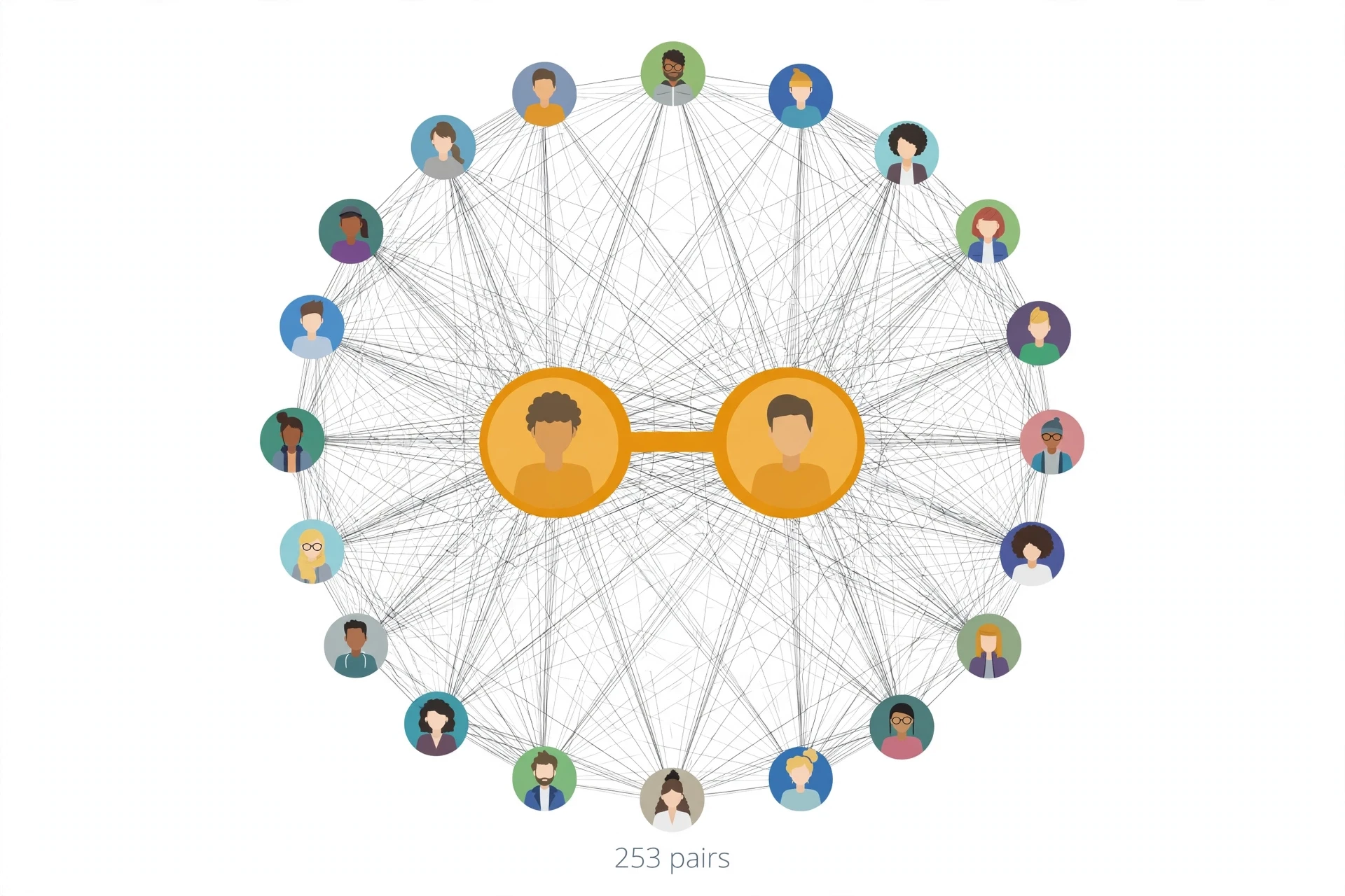
The intuition that says "you need about 180 people" is comparing people with days: twenty-three people against 365 days looks hopeless. The correct comparison is pairs with days: 253 pairs against 365 days looks like a fair fight, and it is. Whenever a probability problem surprises you, check what you are counting. The usual error is counting the wrong thing — people instead of pairs, doors instead of cases, trials instead of combinations.
9.3 The calculation, step by step
The clean way to calculate the birthday probability is through the complement — the chance that nobody shares a birthday — and then subtract from one. The first person can have any birthday: 365 out of 365. The second person must avoid the first person's birthday: 364 out of 365. The third must avoid two birthdays: 363 out of 365. Each new person must avoid all the birthdays taken so far. For twenty-three people, the chance that all birthdays are different is the product of 365/365 times 364/365 times 363/365, all the way down to 343/365. That product is about 0.4927. So the chance that at least two people share a birthday is one minus 0.4927, which is 0.5073, or 50.73%. A clear step-by-step walkthrough of the same calculation is in Unseel's birthday paradox explainer.
The same calculation gives the rest of the table. With thirty people, the chance is about 70%. With forty, about 89%. With fifty, about 97%. With fifty-seven, about 99%. And with 366 people, a match is certain — there are only 365 possible birthdays, so two people must share one. That last fact is the pigeonhole principle, and it is the only part of the problem that needs no probability at all.
The standard calculation makes three simplifying assumptions: 365 possible birthdays, with the 29th of February ignored; every day equally likely; and different people's birthdays independent of each other. Real birthdays are not perfectly uniform — more babies are born in some months than in others — but the non-uniformity only makes matches more likely, not less. A mathematician named D. M. Bloom proved in 1973 that among all possible distributions of birthdays across the days of the year, the uniform one gives the lowest probability of a match. So twenty-three is a worst case. In the real world, the threshold is the same or lower.
9.4 Why matching YOUR birthday is a different problem
Now ask the other question: how many people do you need before it is more likely than not that someone shares your birthday? The answer is about 253 other people — more than ten times as many. With twenty-three people in the room, the chance that someone shares your particular birthday is only about 5.86%. The reason is the same counting as before, running in reverse: your birthday is one fixed day, so there are only twenty-two chances to match it, not 253 pairs. The paradox is not about birthdays. It is about the difference between "someone matches someone" and "someone matches me", and that difference — between an open question and a fixed target — shows up everywhere in probability, from DNA matching to lottery syndicates to the search for extraterrestrial life.
The birthday paradox is also the reason computer security cares about hash collisions. A hash function maps data to a fixed number of possible values, and the same arithmetic says that collisions become likely once the number of items approaches the square root of the number of possible values. With a 365-day year, the square root is about nineteen, and the threshold is twenty-three. The numbers are close because the mathematics is the same. How encryption works explains what hash functions are for; the birthday paradox explains why they need to be so large.
10. Expected Value: What a Chance Is Worth
10.1 The weighted average that prices risk
Expected value is the answer to a practical question: what is a chance worth? If a gamble pays different amounts with different probabilities, its expected value is the average of the payoffs, weighted by their probabilities — the amount you would get per play, on average, if you played forever. It is Huygens' idea from 1657, and it is the single most useful number in applied probability, because it turns a gamble into a price.
Take a simple game. You pay one coin to roll a fair die. If it shows a six, you win six coins; otherwise you win nothing. The expected value of the win is one sixth times six, plus five sixths times zero, which is one coin. You paid one coin to play, so the game is fair: over many plays, you break even on average. If the prize were five coins instead of six, the expected value would be five sixths of a coin, and you would lose about one sixth of a coin per play in the long run. If the prize were twelve coins, you would gain a coin per play on average, and the person offering the game would soon stop offering it.
Notice what expected value does not promise. It does not promise that any single play will pay one coin — no single play of the die game pays one coin; it pays either six or zero. Expected value is a long-run average, and the long run can be very long. A game with a positive expected value can still bankrupt you if you play it once with money you cannot afford to lose. Expected value is a guide to pricing, not a guarantee of outcome, and confusing the two is how people lose money slowly at games they believe they are winning.
10.2 Fair games, good bets, and bad bets
A fair game has expected value zero — neither side gains on average. A good bet has positive expected value for you. A bad bet has negative expected value. Casinos offer only bad bets, and they stay in business because the law of large numbers — section 11 — guarantees that the average will assert itself over thousands of plays, even though any single player can win on a given night. The house edge is the negative expected value, expressed as a percentage of each bet: 2.70% on a European roulette wheel, 5.26% on an American one. Those percentages look small. Over a long evening, they are inexorable.
The same arithmetic prices insurance. An insurer cannot predict whether you, personally, will have a car accident this year. But it can predict, from data on hundreds of thousands of similar drivers, how many accidents there will be in total — and it sets your premium a little above your share of that total. The difference between the premium and the expected payout is the insurer's margin, and the law of large numbers makes the total predictable enough to run a business on. Edmond Halley showed how to do this in 1693, when he built the first life table from the birth and death records of Breslau and used it to price annuities. The mathematics has not changed since; only the data has got better.
10.3 Why the lottery is a tax on bad arithmetic
Now price a lottery ticket. A Powerball play costs two dollars. The jackpot odds are one in 292,201,338, and the smaller prizes add a little more. Even with a jackpot of a hundred million dollars, the expected value of a ticket is well under a dollar — the exact figure depends on the jackpot and on how many other people buy tickets, because a shared jackpot is split. You are paying two dollars for something worth, on average, far less than two dollars. The gap is the lottery's margin, and it is how the game funds its prizes and its good causes.
None of this means you should never buy a ticket. A ticket also buys a daydream, and a daydream has a value that expected value does not measure. What it means is that you should not buy a ticket as an investment, or as a retirement plan, or because a particular set of numbers is "due". No set of numbers is due. Every combination is equally likely, every drawing is independent, and the numbers that won last week are no more and no less likely to win this week than any others. The lottery is a game with a negative expected value and a very large variance: almost everyone loses a little, and one person, very rarely, wins a lot. If you understand that, the ticket is an entertainment purchase. If you do not, it is a tax on bad arithmetic.
11. The Law of Large Numbers: Why Frequencies Settle Down
11.1 The weak law, in plain words
Flip a coin ten times, and you might get seven heads. Flip it a hundred times, and the fraction of heads will probably be between 40% and 60%. Flip it ten thousand times, and it will almost certainly be within a percentage point or two of 50%. That is the law of large numbers: as the number of independent trials grows, the observed frequency closes in on the true probability. Jacob Bernoulli proved the first version of it in Ars Conjectandi in 1713, after working on it for about twenty years, and it is the theorem that connects the two views of probability we met in section 2 — the counting view and the frequency view. The count says the probability of heads is one half; the law of large numbers says the frequency will confirm it, if you flip long enough.
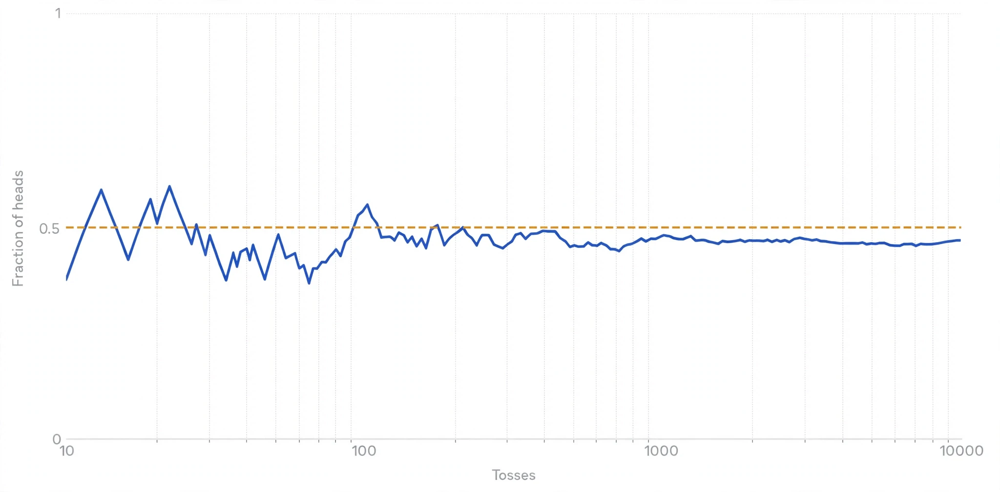
The law is about the fraction, not the difference. After a hundred tosses, you might have fifty-five heads and forty-five tails — a difference of ten. After ten thousand tosses, you might have 5,050 heads and 4,950 tails — a difference of a hundred, ten times bigger. The difference grows, but the fraction — 55% after a hundred tosses, 50.5% after ten thousand — gets closer to one half. The deviations are not cancelled; they are diluted. That distinction is the key to the whole subject, and it is the distinction the gambler's fallacy gets wrong.
11.2 The bell curve and the margin of error in polls
The law of large numbers says the frequency settles down. The central limit theorem says how it settles down: the distribution of the average, over many trials, approaches the bell curve, whatever the underlying distribution was. Abraham de Moivre found the first version in 1733, studying coin tosses; Laplace extended it in 1812; and the theorem is the reason opinion polls can quote a margin of error.
The arithmetic is simple enough to check. Ask a thousand randomly chosen people a yes-or-no question, and the standard deviation of the fraction answering yes is about the square root of (0.25 divided by 1,000), which is about 0.0158, or 1.58 percentage points. The 95% margin of error is about 1.96 times that, or about 3.1 percentage points — the familiar "plus or minus three points" of a thousand-person poll. Ask ten thousand people instead, and the margin shrinks to about one point, because the error shrinks with the square root of the sample size: four times the sample, half the error. That square-root rule is the reason pollsters stop at about a thousand respondents. Going bigger buys very little accuracy for a great deal of money. The full proof of the weak law, and the step from it to the central limit theorem, is laid out in Libre University's lesson on the laws of large numbers.
The same bell curve explains why so many natural measurements — heights, test scores, measurement errors — pile up in the middle and thin out at the edges. When a quantity is the sum of many small independent influences, the central limit theorem says its distribution will be approximately normal, and the approximation gets better as the number of influences grows. It is one of the most useful theorems in all of science, and it is pure probability: no physics, no biology, just the arithmetic of averaging.
11.3 What the law does NOT say: the gambler's fallacy
The law of large numbers is the most misquoted result in mathematics, and the misquotation has a name: the gambler's fallacy. It is the belief that a run of one outcome makes the other outcome "due" — that after five heads, tails is more likely, because the coin must "balance out". The coin must do no such thing. The coin has no memory, no ledger, and no sense of fairness. The probability of heads on the sixth toss is one half, exactly as it was on the first.
What the law actually says is that over a very large number of tosses, the fraction of heads will be close to one half. It does not say that the difference between heads and tails will shrink. If you flip a coin a hundred times and get sixty heads, the law does not predict forty heads in the next hundred to "even it out". It predicts about fifty heads in the next hundred — the same as always — and the total will be about 110 heads out of 200, or 55%, closer to half than 60% was. The early excess is not cancelled. It is diluted by the weight of later tosses. Tversky and Kahneman put it plainly in their 1971 paper Belief in the law of small numbers: people feel that the fairness of the coin entitles them to expect any deviation will soon be cancelled by a corresponding deviation in the other direction. It will not. Deviations are diluted, not cancelled — and the difference between those two words is the difference between understanding probability and being fooled by it.
12. Common Mistakes and Misconceptions
12.1 The gambler's fallacy and the night black hit 26 times
The most famous demonstration of the gambler's fallacy happened at the Monte Carlo Casino on 18 August 1913, when a roulette wheel landed on black twenty-six times in a row. As the run went on, gamblers bet more and more heavily on red, sure that it was "due", and lost heavily — millions of francs, by some accounts. The probability of twenty-six blacks in a row on a European wheel, with eighteen black pockets out of thirty-seven, is (18/37) raised to the power 26, about 7.3 in a billion, or roughly one in 137 million. Either colour running twenty-six times is about one in 68 million. It was a genuinely rare event.
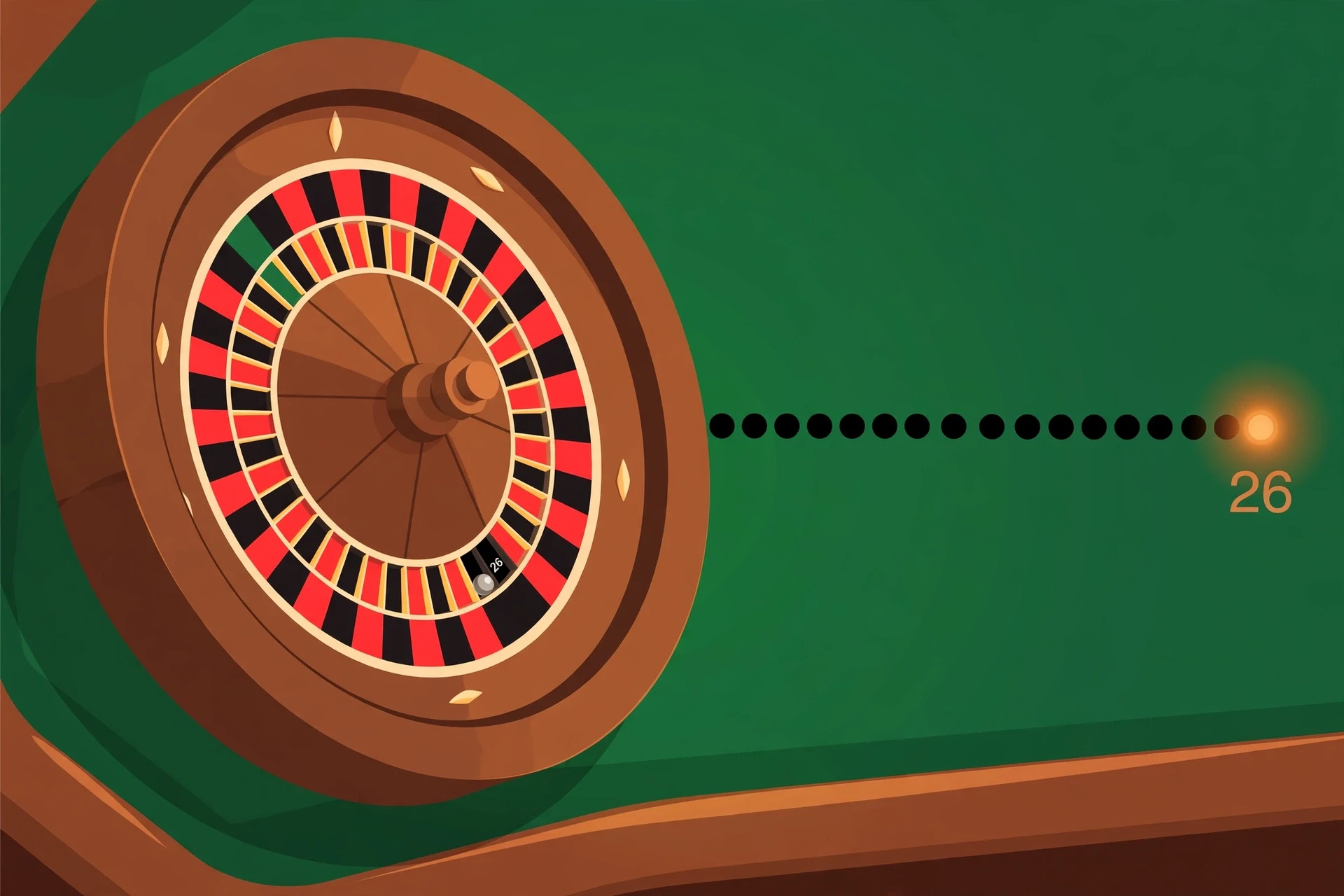
But here is the point the gamblers missed: rarity in advance is not rarity after the fact. Once twenty-five blacks had already landed, the chance of a twenty-sixth black was still 18 in 37, just under a half. The sequence as a whole was extraordinary. The next spin was ordinary. The wheel had no memory of the twenty-five blacks, and no obligation to produce a red. Every spin was a fresh sample space of thirty-seven pockets, and red's eighteen chances were exactly where they had always been.
The fallacy is sometimes called the Monte Carlo fallacy, and it is not confined to casinos. Investors who sell after a run of losses because a recovery is "due", patients who skip a treatment because a side effect is "due" to skip them, and sports fans who expect a missed shot to be followed by a made one are all making the same error: treating independent events as if they shared a memory. The cure is the same in every case. Ask whether the events are independent. If they are, the past is irrelevant, however dramatic it looks.
12.2 "The law of averages" is not a law
You will hear people say "the law of averages" as if it were a theorem of probability. It is not. There is a law of large numbers, and it says what section 11 says: frequencies settle down over many trials. There is no law that says a short run must be balanced by an opposite run, and no law that says a coin, a die, or a roulette wheel owes you anything. The phrase "law of averages" is usually the gambler's fallacy wearing a statistical-sounding name, and it should set off an alarm whenever you hear it.
The confusion is understandable, because the law of large numbers sounds like it promises balance. It does not. It promises dilution, over a long run, of whatever imbalance has already occurred. The difference matters in practice: if you have flipped five heads in a row, the law of large numbers does not make tails more likely next. It makes the fraction of heads over the next thousand flips likely to be near a half — and that fraction includes the five heads you have already seen, as a small and shrinking part of a much larger total.
12.3 Base-rate neglect and the prosecutor's fallacy
Section 7 covered these in detail, so here is the short version. Base-rate neglect is forgetting how common something was before the evidence arrived. A test that is 99% accurate can still be wrong nine times in ten when the disease is rare. The prosecutor's fallacy is confusing the probability of the evidence given innocence with the probability of innocence given the evidence. Both errors come from the same root: treating a conditional probability as if it ran in both directions. It does not. P(A given B) and P(B given A) are different numbers, and the difference between them is often the whole case.
12.4 The hot hand and streaks
The mirror image of the gambler's fallacy is the hot hand: the belief that a run of successes means the next attempt is more likely to succeed, because the player is "hot". In genuinely independent trials — coin tosses, roulette spins — there is no hot hand; the streak is what randomness looks like. Random sequences are clumpy. They contain runs, and the runs feel meaningful, because the human brain is a pattern-finding machine that would rather see a story than a coincidence. Cognitive biases explains why the brain does this, and how we make decisions explains how fast, intuitive thinking produces these judgements before slow, careful thinking gets a chance to check them.
That said, the hot hand is not always a fallacy. In basketball, a player's confidence, rhythm, and the defence's reaction can genuinely change the probability of the next shot — the trials are not independent, because the player is not a coin. The fallacy is assuming a streak proves a hot hand, when randomness alone produces streaks of exactly the same length. The test is independence: if the trials are independent, streaks mean nothing. If they are not, the streak might mean something — but you need evidence beyond the streak itself to say so.
12.5 Confusing probability with odds — and with certainty
Two final confusions, both linguistic. First, probability and odds are different numbers for the same chance, and mixing them up produces wrong answers: a probability of three quarters is odds of three to one in favour, not odds of three to four. Section 13 gives the conversion. Second, a high probability is not certainty. A 99% chance means that in a hundred similar situations, the event fails about once — and if you meet a hundred such situations, you will meet that failure. People who treat a 95% forecast as a promise are surprised, on average, one time in twenty. The surprise is not the forecast's fault. It is the reader's.
"The gambler feels that the fairness of the coin entitles him to expect that any deviation in one direction will soon be cancelled by a corresponding deviation in the other. … Deviations are not canceled as sampling proceeds, they are merely diluted." — Tversky and Kahneman, on the law of small numbers, 1971
13. Probability vs Odds: Two Languages for the Same Idea
13.1 Converting between them
Probability and odds describe the same chance in two different ways, and the conversion is simple once you see it. Probability counts favourable outcomes against all outcomes. Odds count favourable outcomes against unfavourable outcomes. A probability of three quarters means three favourable outcomes out of four total. The odds in favour are three to one — three favourable against one unfavourable. A probability of one in four is odds of three to one against.
The formulas run both ways. If the probability is p, the odds in favour are p divided by (1 − p). If the odds in favour are a to b, the probability is a divided by (a + b). A coin toss at evens — odds of one to one — is a probability of one half. A horse at odds of three to one against has probability one in four, or 25%. A lottery ticket at odds of 292 million to one against has probability one in 292,201,338 — the same number, in a language that makes the payout easy to see and the smallness of the chance easy to miss.
13.2 Why bookmakers speak odds and scientists speak probability
Bookmakers speak odds because odds make the payout visible. Odds of three to one mean: stake one coin, and if you win you get your stake back plus three. Scientists speak probability because probabilities combine cleanly: independent probabilities multiply, mutually exclusive probabilities add, and Bayes' theorem is written in probabilities. Neither language is wrong. The trouble starts when people translate sloppily — when "odds of one in four" is used to mean a probability of one in four (it means one in five), or when a "one in a million chance" is quoted as if it were odds of a million to one (it is odds of 999,999 to one against, which is near enough the same thing that nobody minds, but the sloppiness is a habit worth noticing).
| Probability | As a percentage | Odds in favour | Odds against | Everyday example |
|---|---|---|---|---|
| 1 | 100% | — | — | Certainty |
| 3/4 | 75% | 3 to 1 | 1 to 3 | A biased coin landing heads |
| 1/2 | 50% | 1 to 1 (evens) | 1 to 1 | A fair coin landing heads |
| 1/4 | 25% | 1 to 3 | 3 to 1 | Drawing a heart from a full deck |
| 1/6 | 16.7% | 1 to 5 | 5 to 1 | Rolling a six |
| 1/36 | 2.8% | 1 to 35 | 35 to 1 | Rolling two sixes |
| 1/292,201,338 | 0.0000003% | 1 to 292,201,337 | 292,201,337 to 1 | Winning the Powerball jackpot |
| 0 | 0% | — | — | Impossibility |
14. Where Probability Actually Runs the World
14.1 Weather: what "30% chance of rain" really means
The most familiar probability in daily life is the one on your weather app, and it is also one of the most misunderstood. A "30% chance of rain" does not mean it will rain for 30% of the day. It does not mean rain will fall over 30% of the map. It means, in the definition used by the US National Weather Service, that there is about a three-in-ten chance that at least 0.01 inches of rain — the threshold for "measurable" precipitation — will fall at your location during the forecast period. Put the other way round, it means a seven-in-ten chance of staying dry.
Forecasters calculate it as PoP = C times A: their confidence that rain will occur somewhere in the forecast area, multiplied by the share of the area expected to get it. If a forecaster is certain that rain will develop but expects it to cover only 30% of the area, the chance of rain at your particular spot is 30%. The number bundles confidence and coverage together into a single probability at a point, which is why it is so easy to misread. The probability also says nothing about how hard it will rain. A 30% chance can mean a brief, violent thunderstorm; a 90% chance can mean a light drizzle. Likelihood is not intensity, and probability is not a forecast of how much.
I learned this the way most people do: by getting wet on a "20% chance of rain" day and feeling cheated. The forecast was not wrong. A 20% chance means rain about one time in five, and I had simply met the one. A well-calibrated forecast is right, on average, exactly as often as it claims to be — a 30% forecast should see rain about three times in ten. Judging a probability forecast by a single day is like judging a coin by a single toss. Monsoons, El Niño, hurricanes, and Earth's atmosphere all run on these same forecasting methods, and the probabilities in them are doing the same job: turning the output of many model runs into a single number you can act on.
14.2 Insurance and the business of pricing risk
Insurance is the law of large numbers turned into a business. An insurer cannot predict whether you will have an accident this year, and it does not try. It predicts how many accidents a hundred thousand drivers like you will have, and that number is highly predictable, because the law of large numbers squeezes the uncertainty out of the total even while each individual case stays uncertain. Your premium is your share of that predicted total, plus a margin for running the business. Halley did the first version of this calculation in 1693, with a table of deaths in Breslau. Modern insurers do it with vastly more data and the same mathematics.
The key insight is that pooling changes the risk without changing any individual's chance. One person facing a one-in-a-thousand chance of a ruinous loss is in trouble. A hundred thousand people facing the same chance, each paying a small premium, can cover the thousand losses easily — because the number of losses is predictable, even though which people suffer them is not. That is what insurance sells: not certainty, but the conversion of an unpredictable personal catastrophe into a predictable shared cost. It is probability's oldest commercial application, and still its most important.
14.3 Medicine: tests, screening, and why doctors think in priors
Medicine runs on Bayes' theorem, whether doctors name it or not. A test result is evidence, and evidence updates a prior — the probability of the disease before the test, given the patient's age, symptoms, and history. A positive result on a rare disease means something very different from the same positive result on a common one, as section 7 showed: the same test, the same accuracy, and a wildly different answer, because the base rate changed. Good clinicians think this way instinctively. They ask how common the condition is before they order the test, and they order a second test — a different kind of test, with different failure modes — before acting on a surprising result.
Screening programmes make the same calculation at population scale. Screening a million healthy people for a rare disease will find the few real cases, but it will also produce many more false alarms, and each false alarm costs anxiety, further testing, and sometimes harmful treatment. Whether a screening programme is worth running depends on the base rate, the test's accuracy, and the cost of being wrong in each direction — which is why some screenings are recommended for everyone and others only for people at higher risk. The arithmetic is Bayes' theorem; the decision is about values as well as numbers, and no formula can make it for you. How human brain forms memories and genetic drift both deal with processes where small probabilities compound over many trials, and the same base-rate thinking applies.
14.4 Machines that bet: spam filters, weather models, and AI
The newest home of probability is inside machines. A spam filter is Bayes' theorem in code: it starts with a prior — the fraction of all email that is spam — and updates it with the evidence of each word in the message. The word "lottery" raises the probability of spam; the word "invoice" lowers it; the filter multiplies the evidence together and sorts the message when the updated probability crosses a threshold. It makes mistakes, and the mistakes are the same kinds a human makes: rare words it has never seen, and base rates that shift when a spammer changes tactics.
Weather models run the same idea at a larger scale: many model runs with slightly different starting conditions, and the fraction of runs that produce rain becomes the forecast probability. Machine-learning systems — the subject of how artificial intelligence works — are probability machines through and through: they estimate the probability of each possible next word, each possible classification, each possible move, and choose the most probable, or sample from the distribution. Even GPS uses probability, filtering noisy satellite signals to estimate the most likely position. Probability began as a way to divide the stakes of an interrupted dice game. It has become the language in which machines reason about an uncertain world — and the language in which we should reason about them. That is the answer to the question this article started with — what is probability? — and it is a better answer than the one most people carry around: not a guess, not a feeling, but a number, honestly arrived at, that tells you how much you know.
"Although in games depending entirely upon fortune, the success is always uncertain, yet it may be exactly determined at the same time, how much more likely one is to win than lose." — Christiaan Huygens, opening his 1657 treatise on games of chance
15. Frequently Asked Questions
15.1 What is probability in simple terms?
Probability is a number between zero and one that measures how likely something is. Zero means it cannot happen, one means it is certain, and everything else falls in between. A fair coin landing heads has probability one half. The number summarises what a reasonable person should expect, given what they know — it never predicts a single outcome.
15.2 How do you calculate probability?
When every outcome is equally likely, divide the number of favourable outcomes by the total number of outcomes. A die has six faces, so the chance of a six is one in six. For more complicated problems, count the outcomes with combinations, use the complement rule — calculate the chance that something does not happen and subtract from one — or use conditional probability when new information arrives.
15.3 What is conditional probability?
Conditional probability is the probability of an event given that something else has happened. It is written P(A given B) and calculated as P(A and B) divided by P(B). A card's chance of being a king is one in thirteen, but given that it is a face card, the chance is one in three, because the new information shrank the sample space from fifty-two cards to twelve.
15.4 What is the difference between probability and odds?
Probability counts favourable outcomes against all outcomes; odds count favourable outcomes against unfavourable outcomes. A probability of three quarters is odds of three to one in favour. To convert, use the formulas: odds in favour equal the probability divided by one minus the probability, and probability equals the odds divided by one plus the odds.
15.5 What is the Monty Hall problem?
Three doors hide one car and two goats. You pick a door, the host — who knows where the car is — opens a different door showing a goat, and offers you the chance to switch. Switching wins two times in three; staying wins one time in three. The host's deliberate choice concentrates the two-thirds chance from the doors you did not pick onto the single remaining door.
15.6 Why is the birthday paradox surprising?
In a room of twenty-three people, the chance that two share a birthday is about 50.73% — more likely than not. The surprise is that the question is about any pair matching, and twenty-three people form 253 pairs, each a one-in-365 chance. Matching your birthday is a different question, and takes about 253 other people to reach fifty-fifty.
15.7 What does a 30% chance of rain actually mean?
It means there is about a three-in-ten chance that at least 0.01 inches of rain will fall at your location during the forecast period — and a seven-in-ten chance of staying dry. It does not mean rain for 30% of the day, rain over 30% of the map, or light rain. The number says nothing about how hard it will rain.
15.8 What is Bayes' theorem in simple terms?
Bayes' theorem tells you how to update a belief when new evidence arrives: take what you believed before, multiply by how likely the evidence is under each possibility, and read off the updated odds. Its most famous lesson is the disease-test example — a 99% accurate test for a disease that affects one person in a thousand gives a positive result that means only about a 9% chance of actually being ill, because the disease is rare and false alarms outnumber true cases.
16. Sources
- Encyclopaedia Britannica, Monty Hall problem — https://www.britannica.com/topic/Monty-Hall-problem
- Wikipedia, Bayes' theorem — https://en.wikipedia.org/wiki/Bayes%27s_theorem
- Mathematics LibreTexts, Probability (Sekhon and Bloom, Finite Mathematics) — https://math.libretexts.org/Courses/SUNY_Geneseo/Math_113%3A_Finite_Math_for_Society/09%3A_Probability
- OpenStax, Introductory Statistics — https://openstax.org/books/introductory-statistics-2e
- Utah State University, History of Probability — http://5010.mathed.usu.edu/Fall2020/ENelson/History.html
- Dartmouth, Huygens — The Value of all Chances in Games of Fortune — https://math.dartmouth.edu/~doyle/docs/huygens/huygens/
- Imperial College London, The Law of Large Numbers (Bingham, 2013) — https://www.ma.imperial.ac.uk/~bin06/talks/arsconjIV.pdf
- Libre University, The laws of large numbers — https://en.libre.university/lesson/probability/the-laws-of-large-numbers
- Encyclopaedia Britannica, Edmond Halley — https://www.britannica.com/biography/Edmond-Halley
- Powerball, official prize chart — https://www.powerball.com/powerball-prize-chart
- National Weather Service, What Does Probability of Precipitation Mean? — https://www.weather.gov/lmk/pops
- Unseel, The Birthday Paradox — https://unseel.com/mathematics/birthday-paradox
- Wikipedia, Birthday problem — https://en.wikipedia.org/wiki/Birthday_problem
- Wikipedia, Gambler's fallacy — https://en.wikipedia.org/wiki/Gambler%27s_fallacy
- Wikipedia, Probability axioms — https://en.wikipedia.org/wiki/Probability_axioms
- Stanford Encyclopedia of Philosophy, Interpretations of Probability — https://plato.stanford.edu/entries/probability-interpret/
- Khan Academy, Probability — https://www.khanacademy.org/math/statistics-probability
- Keith Devlin, The Unfinished Game (book, print citation)
- Peter Bernstein, Against the Gods (book, print citation)
- Leonard Mlodinow, The Drunkard's Walk (book, print citation)
- Ian Hacking, The Emergence of Probability (book, print citation)
- Andrey Kolmogorov, Foundations of the Theory of Probability, 1933 (book, print citation)
- Thomas Bayes, An Essay Towards Solving a Problem in the Doctrine of Chances, Philosophical Transactions, 1764 (volume for 1763) (print citation)
- Jacob Bernoulli, Ars Conjectandi, 1713 (print citation)
- Tversky, A., and Kahneman, D., Belief in the law of small numbers, Psychological Bulletin, 76(2), 1971, pp. 105–110 — https://doi.org/10.1037/h0031322