

1. The Speedometer Problem: What Calculus Actually Answers
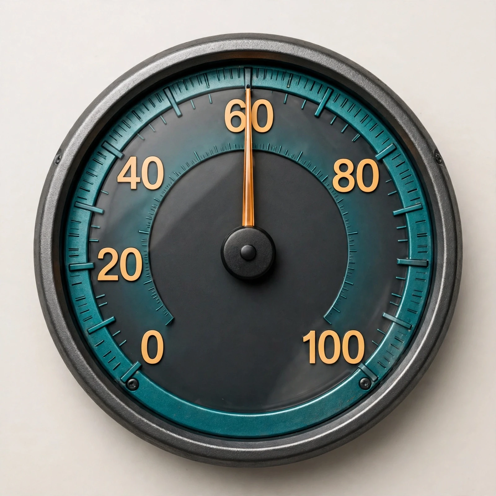
Picture yourself driving along a quiet road at dusk. The headlights pick out the bends ahead, the engine hums, and your eyes flick down to the dashboard. The needle sits at sixty. Sixty what? Sixty miles per hour, right now, at this exact instant. Not your average speed since you left home. Not how far you have travelled. Just this moment, this speed, this second.
Now try to answer a question that sounds simple and turns out to be strangely hard: how fast are you going right now? Speed is distance divided by time, and time is the problem. Over an hour, the calculation is easy. Over a minute, still easy. But "right now" means over no time at all, and distance divided by zero is meaningless. Your speedometer still gives you an answer, sixty, and it is right. How?
That question is the doorway into calculus. Learning how calculus works means learning how mathematicians answer questions about a single instant — how fast, how steep, how much — when the ordinary tools of arithmetic break down the moment time or distance shrinks to zero.
Calculus asks two questions, and the whole subject is built from them. The first is the speedometer question: how fast is something changing at one precise moment? The second is the opposite question: if you know how fast something has been changing all along, how much has it changed in total? How far did the car actually travel, given a speedometer reading that kept moving up and down for an hour? The first question leads to the derivative. The second leads to the integral. And the most startling fact in the subject — the one that makes calculus a single subject instead of two — is that those two questions are secretly the same question asked in reverse.
I remember the first time a teacher wrote the speedometer problem on the board and refused to accept "divide distance by time" as an answer. The class argued for ten minutes. Someone said the speedometer must be averaging over a very short time. Someone else said it must be guessing. The teacher let us argue, then drew a curve on the board and a straight line touching it at one point, and said the speedometer was measuring the steepness of that line. I did not believe her at first. It took me years of teaching the same idea to students of my own before I understood how right she was — and how strange it is that a line touching a curve at a single point can tell you something real about the world.
This article follows that thread from beginning to end. We will start with what calculus is and where it came from, meet the idea of a limit — the quiet trick that makes the whole subject possible — then work through derivatives and integrals with real numbers, not just symbols. We will prove nothing in the formal sense, but we will calculate everything we claim, step by step, so you can check the arithmetic yourself. By the end you will know what a derivative is, what an integral is, how the two are related, and why this mathematics, now more than three centuries old, still runs the modern world, from spacecraft to medical dosing to the algorithms that train artificial intelligence.
2. What Is Calculus? The Mathematics of Change
Calculus is the branch of mathematics that studies change and accumulation. Where arithmetic counts things and algebra solves for unknowns, calculus asks how quantities vary — how fast a population grows, how steeply a hill rises, how much water has flowed through a pipe by the end of the day. If the world stood still, we would never have needed it. It moves, so we did. That is the question at the heart of how calculus works: turning things that change into numbers you can calculate with.
The subject has two branches, and their names tell you what each one does. Differential calculus studies rates of change: slopes, speeds, and how quickly one quantity responds when another one moves. Integral calculus studies accumulation: totals, areas, and volumes built up from tiny pieces. The word "differential" comes from "difference" — a small change. The word "integral" comes from "integer", whole — putting pieces together into a whole.
Here is the difference in one everyday picture. Imagine a water tank with a tap. Differential calculus answers: how fast is the water level rising right now? Integral calculus answers: how much water is in the tank after an hour of filling? The first question is about a rate at an instant. The second is about a total built up over time. They sound like different jobs, and the two problems behind them — finding a tangent and finding an area — were studied separately for centuries before anyone saw they were inverses. The fundamental theorem of calculus, which we will reach in section 9, says they are inverse operations — each one undoes the other — and that discovery is what turned a collection of clever tricks into a single subject.
Most people meet calculus as a school subject full of symbols, and the symbols can make it look harder than the ideas. The core ideas are three, and they fit in one paragraph. A limit describes what happens as something gets closer and closer to a value without necessarily reaching it. A derivative is a limit of a slope: the steepness of a curve at a single point. An integral is a limit of a sum: the total you get by adding up infinitely many infinitely thin slices. Everything else — the rules, the theorems, the applications — is machinery built on those three ideas.
The word "calculus" itself is Latin for a small pebble. Roman merchants counted with pebbles on a board, and the name stuck to the art of calculation long before it attached itself to this particular mathematics. When people in the 1600s began calling the new mathematics "the calculus", they meant something like "the method of calculation" — the calculating engine that could finally handle motion and change. The name was modest. The engine was not.
A fair question at this point: what is calculus not? It is not a different kind of arithmetic, and it does not replace algebra or geometry. It sits on top of them. You cannot do calculus without algebra — every derivative you compute is an algebra problem in disguise — and much of early calculus is geometry with a new idea added. What calculus adds is the handling of the infinite: infinitely small changes, infinitely many pieces, and the precise language of limits that keeps those infinities under control. That is the whole game. If you understand that calculus is algebra and geometry plus limits, you have understood its shape, and the rest of this article is filling in the details.
The standard reference for the subject, used by university courses around the world, is the free textbook Calculus Volume 1 from OpenStax, and the Encyclopaedia Britannica entry on calculus gives a compact account of the same ideas. Both are worth keeping open while you read.
2.1 What is the difference between differential and integral calculus?
This is the question that confuses almost everyone at the start, so it is worth answering plainly before we go further. Differential calculus starts with a quantity and asks how fast it is changing. Give it a distance, and it returns a speed. Give it a temperature, and it returns the rate at which the temperature is rising. Integral calculus starts with a rate and asks how much has accumulated. Give it a speed, and it returns a distance. Give it a flow rate, and it returns a volume.
Think of a bank account. Differential calculus is the statement on your phone that tells you your balance is growing by a certain amount per day. Integral calculus is the total in the account after a year of those daily additions. One describes the flow; the other describes the stock that the flow builds. Neither is more fundamental than the other, and you need both to describe a changing world. By the end of this article you will see exactly how one turns into the other, and why that connection is the deepest idea in the subject.
2.2 Who uses calculus, and who needs it?
Short answer: anyone who works with things that change. Physicists use it to describe motion, from a falling apple to a spacecraft in orbit. Engineers use it to design bridges that flex without breaking and circuits that switch without overheating. Doctors and pharmacologists use it to model how a drug's concentration in the blood rises and falls after a dose. Economists use it to find the price that maximises profit. Computer scientists use it to train the machine learning models behind search engines and chatbots. Biologists use it to model populations, epidemics, and the spread of genes. If a field has rates and totals in it, calculus is somewhere in its toolkit, usually doing the heavy lifting quietly in the background.
You do not need to be any of those people to benefit from understanding it. Calculus is also the clearest window we have into how mathematics grows: a practical problem (how fast? how much?) leads to a new idea (the limit), which leads to a new tool (the derivative, the integral), which leads to a theorem that ties everything together, which leads to a thousand applications nobody foresaw. That arc — problem, idea, tool, theorem, application — is the story of this article.
3. A Very Short History: From Pebbles to Newton and Leibniz
Calculus was not invented in a day. It was assembled over two thousand years, in pieces, by people who did not know they were building the same thing. The story has three acts: the ancient geometers who learned to trap curved quantities between straight ones, the seventeenth-century mathematicians who turned those traps into a method, and the nineteenth-century reformers who finally made the method rigorous.
3.1 The ancient trap: Eudoxus and Archimedes
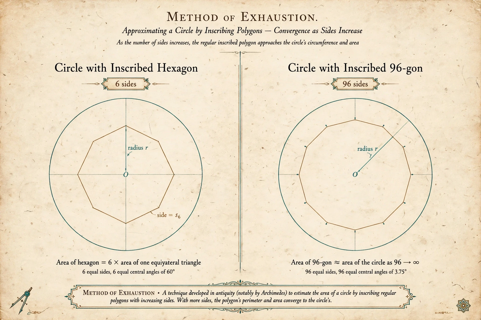
The deepest problem calculus solves is also the oldest: how do you measure something that curves? You can lay rulers end to end along a straight road, but the area inside a circle resists that kind of direct counting. Around 350 BC, Eudoxus of Cnidus offered the first rigorous answer, called the method of exhaustion. Trap the unknown curved quantity between two known quantities — a polygon drawn inside the circle and a polygon drawn outside it — and then make the gap between them as small as you please by using more and more sides. The true area is squeezed between the two estimates, and the squeeze can be made as tight as anyone demands.
Archimedes of Syracuse, working around 250 BC, carried that idea further than anyone would for nearly nineteen centuries. He proved that the area enclosed by a parabola and a chord is exactly four-thirds the area of the inscribed triangle with the same base and height — a result that, in modern language, is a definite integral. He bracketed the value of pi between 3 10/71 and 3 1/7, about 3.1408 and 3.1429, by comparing the circle with inscribed and circumscribed polygons of 96 sides each. He found the surface area and volume of a sphere, and he considered the sphere result — the volume of a sphere is two-thirds the volume of the cylinder that encloses it — his greatest achievement. He is said to have asked for a sphere inside a cylinder to be carved on his tomb.
What makes Archimedes remarkable is not just what he proved but how he found it. In 1906, the Danish scholar Johan Ludvig Heiberg discovered a palimpsest — a manuscript scraped clean and written over — containing a lost work of Archimedes called The Method of Mechanical Theorems. In it, Archimedes admitted that he first discovered his results by imagining figures sliced into infinitely many thin pieces and balanced on a lever, essentially summing infinitesimals, and only afterwards dressed the findings in the rigorous language of exhaustion. He was doing integration in spirit two thousand years early. He never built a general theory of it, though. Each result was proved on its own, by contradiction, and the method stayed a bag of brilliant tricks rather than a machine anyone could use.
3.2 The seventeenth century: two men, one idea, one bitter quarrel
By the 1600s, Europe was ready for a general method. Descartes had joined algebra to geometry, so curves could be described by equations. Fermat had a method for finding the maxima of functions and the tangents to curves. Cavalieri was summing indivisibles. The pieces were lying on the table, and two men picked them up independently and built the machine.
Isaac Newton, working at Cambridge in 1665 and 1666 while the university was closed during the plague, developed his method of fluxions — his name for rates of change, from the Latin for "flowing". He kept it mostly in manuscript, circulating it privately among a small circle, and published his great work on motion and gravity, the Principia, in 1687 with the calculus largely hidden inside geometric arguments. Gottfried Wilhelm Leibniz, a German philosopher and diplomat working in Paris and Hanover, developed his own version from 1675 and published first: a short paper, Nova Methodus pro Maximis et Minimis, in the journal Acta Eruditorum in 1684. It was only about six pages long, dense, and hard to read — but it contained the differential calculus, and Leibniz followed it with the integral calculus.
Then came the quarrel. Newton's supporters accused Leibniz of copying Newton's unpublished ideas. Leibniz's supporters accused Newton of jealousy. The dispute simmered from 1699 and broke out in full force around 1711. In 1712 the Royal Society set up a committee to settle the question of priority, and the committee's report, published as the Commercium Epistolicum and dated 1712, found in favour of Newton — a verdict somewhat weakened by the fact that Newton himself, as president of the Royal Society, had written the report. Leibniz died in 1716 with the dispute unresolved.
The modern verdict, accepted by historians of mathematics, is that both men discovered calculus independently. The evidence is in the approaches themselves: they are genuinely different routes to the same destination. Newton's calculus grew out of physics — flowing quantities, velocities, motion. Leibniz's grew out of geometry and infinite series, and his notation was far better. We still use Leibniz's notation today: dy/dx for a derivative, and the long S-shaped integral sign ∫, which Leibniz introduced as a stretched-out letter S for "sum". Newton used dots over letters for his fluxions, a notation that died out except in physics, where a dot over a letter still means a rate of change with respect to time. The quarrel was ugly, and it split British and continental mathematics for a century, but the mathematics survived it. The fullest account of the dispute is in the MacTutor history of the development of calculus.
"The dispute was bitter, personal, and ultimately pointless as a question of mathematics. Two men reached the same summit by different paths, and the mountain did not care who arrived first."
One detail deserves emphasis, because it is often missed. James Gregory, a Scottish mathematician, had already published a rudimentary geometric form of the fundamental theorem in 1668, before either Newton or Leibniz had their full systems. The theorem was in the air. What Newton and Leibniz did was turn it from a curiosity into a method — a set of rules anyone could learn and apply to new problems. That is the difference between a discovery and an invention, and calculus was both.
3.3 The clean-up: rigour in the 1800s
For a hundred and fifty years after Newton and Leibniz, calculus worked brilliantly and rested on shaky foundations. Mathematicians spoke of "infinitely small" quantities, divided by them, and then set them to zero — a procedure that looks, to a strict logician, like dividing by zero and hoping nobody notices. It worked because the answers were right, but nobody could say exactly why.
In the 1800s, Augustin-Louis Cauchy and Karl Weierstrass rebuilt the subject on the idea of the limit, with a precise definition that banished the infinitely small from the foundations. Instead of saying "let h be infinitely small", they said: a limit is a promise. You tell me how close you want to get, and I can find a small enough step that gets you that close. That definition — the epsilon-delta definition, named for the Greek letters it uses — is the rigorous backbone of every calculus course today. It is also, honestly, the part of the subject that most students find hardest on first meeting. The good news is that you can understand everything in this article with an intuitive picture of a limit, and the rigorous version is there waiting when you want it.
4. The Idea Under Everything: Limits
Every idea in calculus is a limit in disguise. The derivative is a limit of slopes. The integral is a limit of sums. So before we touch either one, we need to understand what a limit is — not as a formula, but as an idea you can feel. Limits are the first piece of how calculus works, and the other two pieces are built on them.
4.1 Zeno's runner and the tortoise
Around 450 BC, the philosopher Zeno of Elea posed a puzzle that still stops people in their tracks. Achilles, the fastest runner in Greece, races a tortoise, and the tortoise is given a head start. By the time Achilles reaches the tortoise's starting point, the tortoise has moved a little further on. By the time Achilles reaches that new point, the tortoise has moved a little further still. The gap keeps shrinking, but it never seems to close — so how does Achilles ever catch the tortoise?
The puzzle survives only through Aristotle's account of it, and philosophers still argue about exactly what Zeno meant. The mathematical answer, though, is clear, and it is the founding idea of calculus. The gaps form a shrinking sequence — half the gap, then a quarter, then an eighth — and the sum of infinitely many ever-shrinking steps can be a finite number. The series 1 + 1/2 + 1/4 + 1/8 + ... adds up to exactly 2, even though it never stops. Achilles catches the tortoise because the total time needed is the sum of that series, and the sum is finite. Infinity is not the same as endlessness without end; sometimes an infinite process has a definite destination. That destination is the limit.
The Stanford Encyclopedia of Philosophy gives the fullest careful treatment of Zeno's paradoxes, including the argument that the paradox is really about whether space and time are infinitely divisible. For our purposes, the runner is enough: the limit is the value a process approaches, even if the process never arrives there in a finite number of steps.

4.2 Approaching without arriving: 0.999... equals 1
The most famous limit in everyday mathematics is also the most disbelieved. Write out 0.999..., the decimal that goes on with nines forever. It looks smaller than 1. It feels smaller than 1. It is exactly equal to 1.
Here is why. Look at the sequence 0.9, 0.99, 0.999, 0.9999, and so on. Each step is closer to 1 than the last, and the distance to 1 shrinks by a factor of ten each time. There is no gap left over at the end, because the process has no end, and the limit of the sequence — the value it is homing in on — is 1. A neat piece of algebra says the same thing: call the number x, so x = 0.999...; then 10x = 9.999...; subtract, and 9x = 9, so x = 1. The algebra is a shortcut. The limit is the reason the shortcut is honest.
This is the point that trips up most beginners, so it is worth saying plainly: a limit describes where a process is heading, not where it has been. The sequence 0.9, 0.99, 0.999, ... never contains the number 1. Its limit is 1 anyway. That gap between "the terms" and "the limit" is exactly what lets calculus divide by something that tends to zero without ever dividing by zero. We will use that trick in the very next section, and it is the trick that makes the derivative possible.
4.3 The limit as a promise
Here is the intuitive version of the rigorous definition, and it is the version to carry in your head. To say "the limit of f(x) as x approaches a is L" means: you can make f(x) as close to L as you like, simply by taking x close enough to a. It is a promise with two parts. You name a tolerance — how close is close enough? — and the function delivers, provided you move x near enough to a. The smaller your tolerance, the closer x has to be, but the promise never breaks.
That is all a limit is. It is not magic, and it is not a guess. It is a precise statement about closeness, and it is strong enough to support the whole subject. When we compute a derivative in the next section, we will take a limit of a slope, and the promise is what guarantees the answer is exact, not approximate. Calculus is exact mathematics built on the idea of getting arbitrarily close. That sounds like a contradiction. It is the central, beautiful contradiction of the subject, and it resolves the moment you accept that "arbitrarily close" can be made precise.
4.4 Why limits come first
Students often ask why a calculus course starts with limits instead of jumping straight to derivatives. The answer is that the derivative is a limit, and without the limit you cannot say what a derivative is — you can only gesture at it. Every rule you will ever learn for differentiating a function is a shortcut for a limit computation, proved once and then used forever. The limits chapter is the foundation; the rest of the building stands on it. If limits feel strange at first, that is normal. They felt strange to the mathematicians of the 1700s too, and it took a century to make them rigorous. Give them time, work the examples, and the strangeness fades into familiarity — usually right around the moment you compute your first derivative from the definition and watch the answer come out clean.
5. Derivatives: How Fast Is It Changing Right Now?
We are ready for the first half of calculus. A derivative measures how fast a quantity is changing at one instant. It is the slope of a curve at a point, the reading on the speedometer, the steepness of the hill exactly where you are standing. Everything in this section is one idea — the slope of a tangent line — worked out carefully with real numbers.
5.1 From secant to tangent
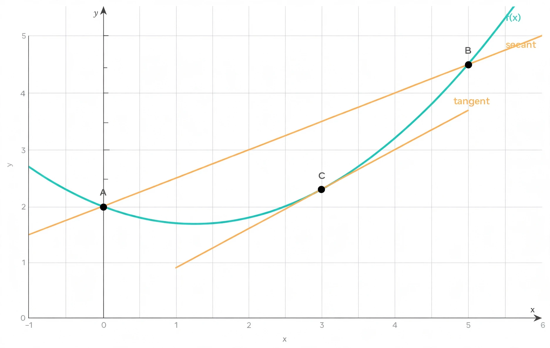
Draw a smooth curve on a page. Pick two points on it and draw the straight line through both. That line is called a secant, and its slope is easy to compute: rise over run, the change in height divided by the change in horizontal distance. It is the average rate of change between the two points — the average speed over a stretch of road.
Now slide the second point along the curve toward the first. The secant line tilts. As the two points get closer, the secant settles down, and in the limit — when the two points merge into one — it becomes the tangent line, the straight line that just touches the curve at that single point and shares its steepness there. The slope of that tangent line is the derivative.
Notice what happened. The average rate of change is easy and slightly wrong: it describes a stretch, not a moment. The instantaneous rate of change is what we want, and it is a limit: the limit of the average rates as the stretch shrinks to nothing. That is the whole definition, and every derivative you will ever meet is this same move, applied to a different curve.
5.2 The difference quotient, in words
Mathematicians write the definition with a formula, and it is worth meeting it once, in plain language, because every textbook will use it. Take a function f, and a point a where you want the slope. Move a tiny distance h away from a, and measure how much the function changed: f(a + h) minus f(a). Divide that change by h. That ratio — change in the function divided by change in the input — is called the difference quotient, and it is the slope of the secant line between the two points. Then let h tend to zero. The limit of the difference quotient, if it exists, is the derivative, written f'(a) or dy/dx.
The notation dy/dx is Leibniz's, and it is worth reading it the way he meant it: a ratio of two tiny changes, dy divided by dx, in the limit as both shrink to nothing. The notation is not just shorthand; it is a hint about how the subject works, and it behaves like a fraction in many calculations, which is one reason it survived for three centuries while Newton's dot notation faded outside physics.
5.3 A worked example: the derivative of x squared
Let us compute a real derivative from the definition, step by step, so you can see the limit do its work. Take f(x) = x squared, the simplest curving function there is, and ask for its slope at the point x = 3.
First, the difference quotient. f(3 + h) is (3 + h) squared, which expands to 9 + 6h + h squared. Subtract f(3), which is 9, and you get 6h + h squared. Divide by h, and you get 6 + h. That is the slope of the secant line between x = 3 and x = 3 + h, and it depends on h: if h is 1, the slope is 7; if h is 0.1, the slope is 6.1; if h is 0.01, the slope is 6.01.
Now take the limit as h tends to zero. The term h vanishes, and the slope settles at exactly 6. The derivative of x squared at x = 3 is 6. And the same calculation at any point x gives the same pattern: the difference quotient is 2x + h, and the limit is 2x. So the derivative of x squared is 2x — the rule you will meet in every textbook, derived here from scratch, with no step hidden.
Check the answer against intuition. The curve y = x squared gets steeper as x grows: at x = 0 it is flat, at x = 1 the slope is 2, at x = 3 the slope is 6, at x = 10 the slope is 20. The derivative 2x says exactly that, and it says it in one short expression. That is the power of the derivative: a whole curve's worth of steepness, captured in a single formula.
5.4 The speedometer, revisited
Return to the car. Suppose the distance you have travelled after t hours is given by a function s(t). Your average speed between two times is the change in distance divided by the change in time — a secant slope. Your speed right now is the limit of those averages as the time interval shrinks — a tangent slope, a derivative. The speedometer in your car is, in effect, a derivative-measuring machine. It does not know the future, and it does not average over the past. It reports the rate of change of distance at this instant, and calculus is the mathematics that says what "at this instant" means.
Acceleration is the same idea applied twice. Velocity is the derivative of distance. Acceleration is the derivative of velocity — the rate at which the speed itself is changing. When you press the accelerator, the speedometer needle climbs; the rate at which it climbs is your acceleration. That is why electric cars, which deliver their torque instantly, feel so quick off the line: their acceleration at the first instant is high, and the electric car article explains how the motor makes that possible. The derivative turns a feeling — "this car pulls hard" — into a number.
5.5 When a derivative does not exist
Not every curve has a tangent at every point, and the exceptions are instructive. A curve with a sharp corner — the absolute value function at zero, like a V — has no single tangent there, because the slope coming in from the left is minus one and the slope coming in from the right is plus one, and no limit can reconcile them. A curve with a jump, or a vertical tangent, fails the same way. When the limit of the difference quotient does not exist, the function is not differentiable at that point.
This is not a defect in the theory. It is the theory telling you something real: at a sharp corner, "how fast is it changing right now" has two different answers depending on which side you approach from, so there is no single answer. Most functions you meet in science are smooth enough to differentiate everywhere that matters, but the exceptions keep the definition honest, and they are the reason the definition is written as a limit in the first place.
6. The Rules That Do the Work: Power, Product, Quotient, Chain
Computing every derivative from the definition would be exhausting. The limit calculation we did for x squared took a paragraph; imagine doing it for a function with five terms, a quotient, and a square root. Nobody does that. Instead, mathematicians proved a handful of rules once, from the definition, and now everyone uses the rules. Four of them do most of the work in a first course. These rules are the working machinery of how calculus works in practice.
6.1 The power rule
The power rule says: the derivative of x to the power n is n times x to the power n minus one. We proved it for n = 2 in the last section: the derivative of x squared is 2x. The same pattern holds for every power. The derivative of x cubed is 3x squared. The derivative of x to the power 10 is 10x to the power 9. The derivative of x itself — x to the power 1 — is 1 times x to the power 0, which is 1: a straight line with slope 1, as it should be. The derivative of a constant is zero, because a constant never changes.
Worked example: f(x) = x to the power 5 plus 3x squared. Differentiate term by term. The derivative of x to the power 5 is 5x to the power 4. The derivative of 3x squared is 3 times 2x, which is 6x. So f'(x) = 5x to the power 4 plus 6x. At x = 1, that is 5 + 6 = 11. One rule, applied twice, and the whole computation takes seconds.
6.2 The product rule and the quotient rule
When two functions are multiplied, their derivatives do not simply multiply. The product rule says: the derivative of f times g is f' times g plus f times g'. Each function takes a turn being differentiated while the other one waits. The intuition is sound: if both factors are growing, the product grows for two reasons at once, and the rule adds the two contributions.
Worked example: f(x) = x squared times sin x. The derivative of x squared is 2x, and the derivative of sin x is cos x. The product rule gives f'(x) = 2x times sin x plus x squared times cos x. At x = 0, sin 0 is 0 and cos 0 is 1, so f'(0) = 0. The curve passes through the origin flat — which makes sense, since x squared is flat there and sin x is small there.
The quotient rule handles division: the derivative of f divided by g is (f' times g minus f times g') divided by g squared. The minus sign is the part everyone forgets, and the mnemonic that saves it is "low d-high minus high d-low, over low squared" — low meaning the denominator, high the numerator. Worked example: f(x) = x divided by (x + 1). The derivative is (1 times (x + 1) minus x times 1) divided by (x + 1) squared, which simplifies to 1 divided by (x + 1) squared. At x = 0 that is 1, and the function is climbing steadily there, which matches the graph.
6.3 The chain rule
The chain rule handles functions inside functions — and most real-world functions are functions inside functions. It says: to differentiate f(g(x)), differentiate the outer function, leave the inner function alone, then multiply by the derivative of the inner function. Peel the onion from the outside in.
Worked example: f(x) = (x squared + 1) to the power 3. The outer function is "cube it"; the inner function is x squared + 1. Differentiate the outside: 3 times (x squared + 1) squared. Multiply by the derivative of the inside: 2x. So f'(x) = 6x times (x squared + 1) squared. At x = 1, that is 6 times 4, which is 24. Without the chain rule you would have to expand the cube first — a mess of algebra. With it, the calculation is two steps.
My own first encounter with the chain rule was a disaster. I tried to memorise it as a formula and kept forgetting whether to multiply by the inner derivative or the outer one. What fixed it was a physical picture: a gear turning a gear turning a gear. The rate at which the last gear turns is the product of the rates at each step, and the chain rule is the same idea written in algebra. If you ever forget the rule, think of the gears.
6.4 A table worth keeping
Here are the derivatives you will use most often, all in one place. Keep it beside you while you read the rest of the article — every worked example from here on uses entries from this table.
Function f(x) | Derivative f'(x) | Where it comes from |
|---|---|---|
x to the power n | n times x to the power n minus 1 | Power rule |
sin x | cos x | Limit of the difference quotient |
cos x | minus sin x | Limit of the difference quotient |
e to the power x | e to the power x | The exponential is its own derivative |
ln x (natural log) | 1 divided by x | Inverse of the exponential |
a constant c | 0 | Constants never change |
Two entries in that table deserve a second look. The exponential function e to the power x is its own derivative — and, up to a constant multiple, the only function with that property: any function satisfying f′ = f is a constant multiple of e to the power x — which is why it appears everywhere growth is involved, from populations to compound interest to radioactive decay. And the derivative of ln x is 1/x, which is why the natural logarithm is the right logarithm for calculus, and why the integral of 1/x is ln x (for x greater than zero). These are not coincidences. They are the same fact seen from two sides, and the fundamental theorem is what connects them.
7. What Derivatives Are For: Peaks, Valleys, and Best Choices
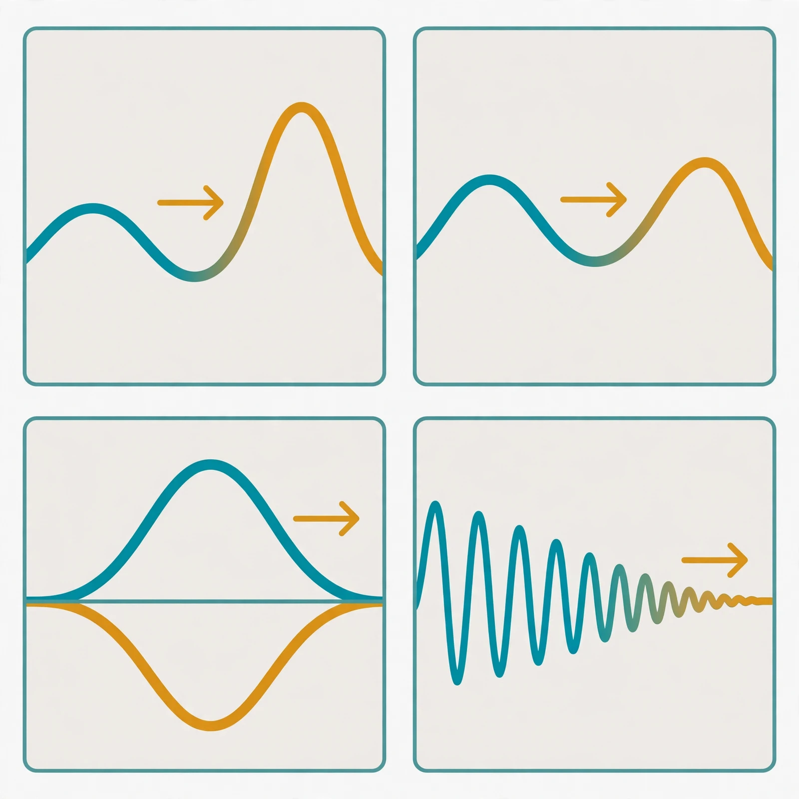
Derivatives are not just a parlour trick for finding slopes. Their real power is that they locate the best and worst of things: the highest point, the lowest point, the cheapest design, the fastest route. That is why engineers and economists reach for them constantly. If you want the maximum of something, find where its derivative is zero.
7.1 Why zero derivative means a peak or a valley
Picture a hill. As you climb, the slope is positive. At the very top, the ground is flat for an instant — the slope is zero. As you descend, the slope turns negative. The top of the hill is exactly where the derivative changes sign from positive to negative, and at that crossing point the derivative is zero. The same logic works upside down for a valley: the slope goes from negative to positive, crossing zero at the bottom.
This gives a practical recipe for optimisation, called the first derivative test. To find the maximum or minimum of a function, differentiate it, set the derivative equal to zero, and solve. The solutions are the critical points, the candidates for peaks and valleys. Then check each one — by looking at the sign of the derivative on either side, or by the second derivative — to see which kind it is. A zero derivative does not guarantee a peak or a valley; a flat stretch of road can also have zero slope without being a summit. But every smooth peak and every smooth valley has a zero derivative at its top or bottom, and that is enough to find them all.
7.2 The fence problem, worked end to end
Here is the classic optimisation problem, worked out in full. You have 100 metres of fencing, and you want to enclose a rectangular garden beside a straight river. The river fences one side for free, so you only need to fence three sides: two short sides running back from the river, and one long side parallel to it. What shape gives the greatest area?
Call the side along the river x, and the depth back from the river y. The fencing used is x plus 2y, and that must equal 100, so x = 100 − 2y. The area is x times y, which becomes (100 − 2y) times y, or 100y − 2y squared. Differentiate with respect to y: the derivative is 100 − 4y. Set it to zero: y = 25. Then x = 100 − 50 = 50. The best rectangle is 50 metres along the river and 25 metres deep, and its area is 50 times 25, which is 1,250 square metres.
Check that it is a maximum, not a minimum: the second derivative of the area is minus 4, which is negative, and a negative second derivative means the curve bends downward — a peak. Also check the edges: if y is 0 or 50, the area is zero, so the interior answer of 1,250 is genuinely the best. The result is also pleasantly symmetric in a way worth remembering: the best rectangle uses exactly half the fencing on the side parallel to the river and a quarter on each of the other two sides. That pattern — spend half on the long side — holds for any amount of fencing, not just 100 metres.

7.3 Related rates: when everything moves at once
A second family of problems asks about rates that are linked. A ladder slides down a wall; how fast is its foot moving when the top is a certain height? A balloon is inflated; how fast is its radius growing when its volume is increasing at a known rate? A shadow lengthens as a person walks away from a lamp; how fast is the tip of the shadow moving?
The method is always the same. Write down the equation that links the quantities — Pythagoras for the ladder, the volume formula for the sphere — then differentiate the whole equation with respect to time. Every quantity that changes contributes a term with its own rate in it, and the chain rule supplies the links. Then plug in the numbers you know and solve for the rate you want. The calculus is short; the hard part is setting the problem up correctly, and the most common error is plugging in numbers before differentiating, which freezes quantities that are still moving.
Take the balloon. Its volume is four-thirds times pi times the radius cubed. Differentiate with respect to time, and the rate of change of volume equals four times pi times the radius squared times the rate of change of the radius. If air is pumped in at a steady rate and the radius is known, the rate at which the radius grows falls out immediately — and it shrinks as the balloon gets bigger, which matches what you see: a nearly full balloon grows in radius much more slowly than a small one for the same puff of air. That is related rates doing what it does best: turning a picture of moving parts into a single equation.
7.4 Concavity and the second derivative
Differentiate once and you get the slope. Differentiate again and you get the second derivative, which measures how the slope itself is changing — whether the curve is bending upward or downward. A positive second derivative means the curve bends upward, like a cup, and the slope is increasing. A negative second derivative means it bends downward, like a hill, and the slope is decreasing. The point where the bending changes direction, where the second derivative crosses zero, is called an inflection point.
This matters in practice because it distinguishes a maximum from a minimum without checking signs on both sides. If the first derivative is zero and the second derivative is negative, you are on a hilltop: a maximum. If the first derivative is zero and the second derivative is positive, you are in a valley: a minimum. In economics, the second derivative tells you whether returns are diminishing. In physics, the second derivative of position is acceleration — the quantity we met in section 5.4 — so the second derivative is the language in which Newton's laws are written. A curve's bending is not decoration; it is information.
8. Integrals: Adding Up an Endless Number of Tiny Pieces
Now the second half of calculus. If the derivative is about zooming in on a single instant, the integral is about zooming out and adding everything up. It answers the opposite question: given a rate that keeps changing, how much has accumulated in total?
8.1 Area under a curve
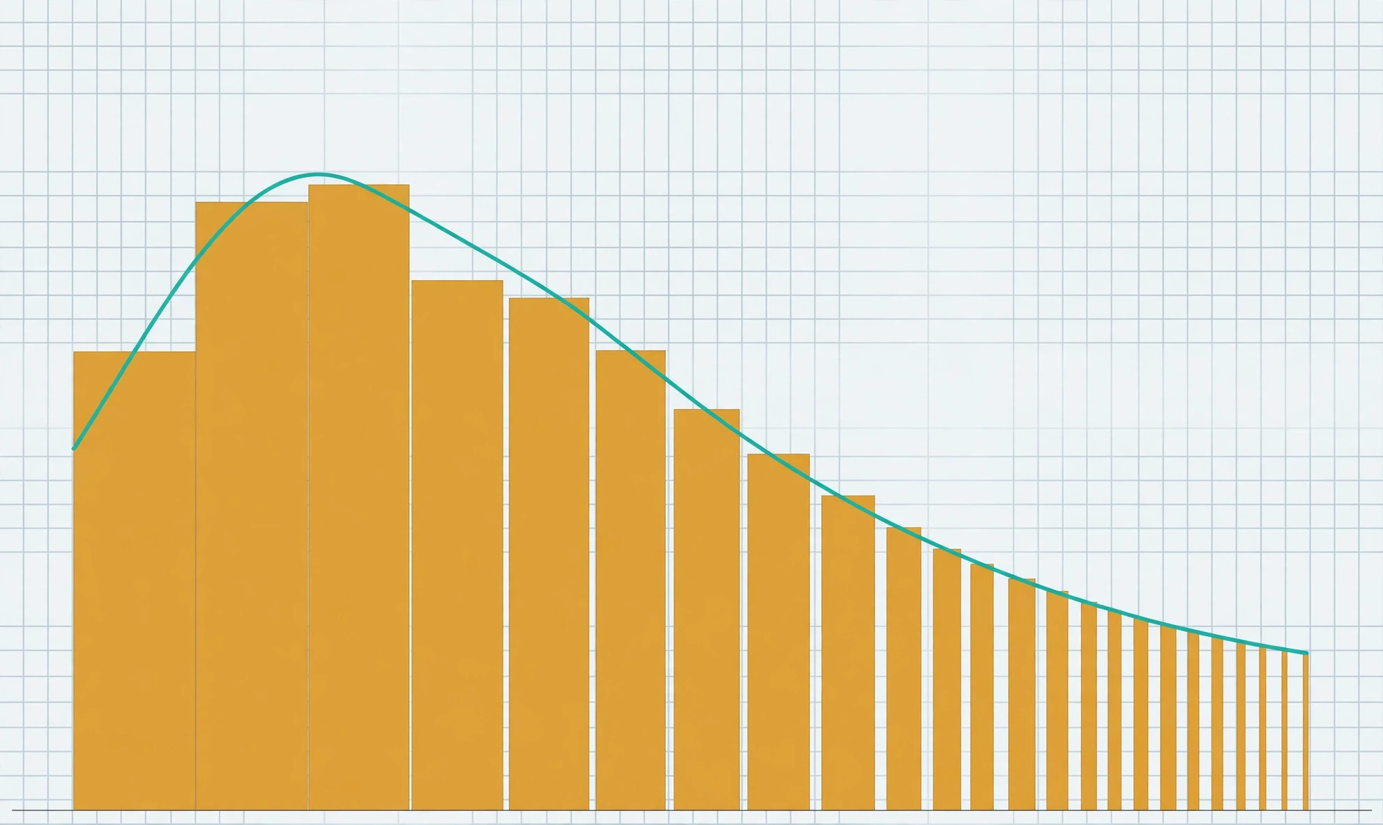
The standard picture is area. Take a curve above the horizontal axis, between two vertical lines, and ask for the area between the curve and the axis. For a rectangle the answer is easy; for a curve it is not, because the height keeps changing. The integral is the answer, and the way to it is slicing.
Slice the region into thin vertical strips, so thin that each one is almost a rectangle. The area of each strip is roughly its height — the value of the function at that point — times its width. Add up all the strips. The result is an approximation, and the thinner the strips, the better it is. Now let the width of the strips tend to zero and the number of strips tend to infinity. The limit of those sums is the definite integral, and it is the exact area. The symbol ∫ is Leibniz's stretched-out S, for "sum", and the dx beside it is a reminder of the width of the strips that shrank to nothing.
This slicing idea is the integral in miniature, and it is older than calculus itself. It is Archimedes' method of exhaustion with the limit made explicit: instead of doubling polygons a few times and stopping, you let the number of pieces grow without bound and ask what the total approaches. The picture to keep is Figure 7 — rectangles under a curve, getting thinner from left to right, homing in on the exact area.
8.2 Riemann sums, with numbers
Let us make the slicing concrete with a small calculation. Take the function f(x) = x squared, between x = 0 and x = 3, and estimate the area under it with three rectangles of equal width. The interval is 3 units wide, so each rectangle is 1 unit wide. Use the right-hand end of each strip for the height: at x = 1 the height is 1, at x = 2 it is 4, at x = 3 it is 9. The areas are 1 times 1, 4 times 1, and 9 times 1 — a total of 14. That is an overestimate, because the curve rises and the right-hand height is the tallest part of each strip.
Use the left-hand ends instead: heights 0, 1, and 4, total 5. That is an underestimate. The true area lies between 5 and 14 — a wide bracket, but a bracket. Now use six rectangles of width one-half, and the bracket tightens. Use a hundred rectangles, and it tightens further. In the limit, as the width tends to zero, the bracket closes on a single number. We will compute that number in the next section with a tool that avoids the slicing entirely — but the slicing is what the number means, and it is worth remembering that every integral is, at heart, a sum of thin pieces.
The sums are called Riemann sums, after Bernhard Riemann, who gave the first careful definition of the integral in the 1850s. The key point of his definition is that the limit must come out the same no matter how you choose the sample points inside each strip — left end, right end, middle, anywhere. For the well-behaved functions of a first course, it always does, which is why the integral is a reliable tool and not a matter of taste.
8.3 Definite and indefinite integrals, and the constant C
Two kinds of integral share a name and a symbol, and confusing them is the most common source of errors in a first course, so here is the distinction stated plainly.
A definite integral has limits — numbers at the bottom and top of the ∫ sign — and it is a number. The integral of x squared from 0 to 3 is a single number, the area we were estimating above. An indefinite integral has no limits, and it is a function: the antiderivative, the function whose derivative is the thing you started with. The indefinite integral of 2x is x squared, because the derivative of x squared is 2x. But it is also x squared plus 5, and x squared minus 17, because the derivative of any constant is zero, so constants vanish on differentiation and reappear on integration as an unknown. That unknown is written as plus C, the constant of integration, and forgetting it is the classic beginner's error. The indefinite integral is not one function but a whole family of functions, all parallel copies of each other, differing by a constant.
Why does the same symbol serve both jobs? Because the fundamental theorem — the subject of the next section — says the two jobs are the same job done in opposite directions. The definite integral, an area computed by slicing, can be evaluated by finding an antiderivative. The antiderivative, a function found by differentiating backwards, computes areas. One symbol, two faces, one theorem joining them.
8.4 A worked example: the integral of x squared
Let us compute the area under y = x squared from 0 to 3, the number our Riemann sums were bracketing between 5 and 14. The antiderivative of x squared is x cubed over 3, by the power rule run backwards: the derivative of x cubed over 3 is 3x squared over 3, which is x squared. Evaluate it at the top limit, 3: 27 over 3 is 9. Evaluate it at the bottom limit, 0: 0. Subtract: 9 minus 0 is 9. The exact area is 9.
Check it against the bracket. Our three-rectangle right-hand estimate was 14, the left-hand estimate was 5, and 9 sits between them, closer to the middle than either. With six rectangles the estimates would be nearer to 9, and with a hundred nearer still. The answer also has the right feel: the average height of x squared over the interval 0 to 3 is 3 — the area 9 divided by the width 3 — and the function's values run from 0 to 9, so an average of 3 is plausible for a curve that spends most of its time low and rises steeply at the end. Every integral you compute should get this kind of sanity check. If the number is outside the bracket your rectangles gave you, something went wrong.
9. The Fundamental Theorem of Calculus: The Two Halves Are One
We have built two machines. One takes a function and returns its rate of change. The other takes a function and returns the total accumulated under it. They look unrelated — one zooms in, the other adds up — and for centuries they were studied separately. The fundamental theorem of calculus says they are inverse operations, each one undoing the other, and it is the single most important theorem in the subject. It is also the reason we could compute the area under x squared in section 8.4 without slicing anything.
9.1 Part 1: differentiate the accumulation, get the function back
Define a new function A(x): the area under the curve of a continuous function f, accumulated from a fixed starting point a up to a moving point x. As x moves right, area accumulates; as x moves left, it drains away. How fast does the accumulated area grow? Think about it physically. At the point x, the curve has height f(x). Move x a tiny step further, and you add a thin strip of area, roughly f(x) times the step. So the rate at which the area grows is f(x) itself. In symbols — whenever f is continuous — the derivative of A is f. Differentiating an accumulation returns the original function.
That is Part 1 of the fundamental theorem: if you build a function by accumulating area under f, then differentiate the result, you get f back. Integration followed by differentiation returns you to where you started. The operation that adds things up is undone by the operation that measures rates of change.
9.2 Part 2: evaluate with a single subtraction
Part 2 is the one you will use a thousand times. If F is any antiderivative of f — any function whose derivative is f — then the definite integral of f from a to b is F(b) minus F(a). The area under the curve, which would take infinitely many rectangles to add up directly, is found by evaluating one function at two points and subtracting. The constant C that haunts the indefinite integral cancels in the subtraction, which is why you can ignore it for definite integrals.
Our worked example from section 8.4 was Part 2 in action. The antiderivative of x squared is x cubed over 3. Evaluate at 3 and at 0, subtract, and the area 9 appears — no rectangles, no limits, no slicing. The miracle is not that the arithmetic is easy; the miracle is that the arithmetic gives the area at all. A rate-of-change machine, run backwards, computes a total. That is the content of the theorem, and it is why calculus became the working tool of science rather than a curiosity: it turned hard problems (areas, volumes, totals) into easy problems (find an antiderivative, subtract twice).
The free OpenStax textbook states both parts carefully in section 5.3, The Fundamental Theorem of Calculus, with the same two-part structure used here.

9.3 Why the theorem matters more than any single calculation
Step back and look at what the theorem does. Before it, computing an area meant summing an infinite series of rectangles, a job so hard that Archimedes could do it only for a handful of shapes, each one a separate triumph. After it, computing an area means finding an antiderivative — and antiderivatives can be found by running the derivative rules backwards, a skill that can be taught in weeks. The theorem turned a research problem into homework.
That pattern — a hard problem becoming easy once the right connection is seen — is the most exciting thing in mathematics, and the fundamental theorem is its purest example. It also explains the structure of every calculus course: differentiation first, because you need the rules before you can run them backwards; integration second, because it leans on everything differentiation taught you; the theorem in the middle, joining them. If you remember one sentence from this article, make it this one: the derivative and the integral undo each other. That single sentence is the heart of how calculus works.
"The fundamental theorem does not just connect two operations. It tells you that the two questions calculus asks — how fast, and how much — are the same question asked in opposite directions."
10. Differential vs Integral Calculus: Side by Side
By now you have met both branches in detail. Here they are side by side, so the contrast is easy to hold in your head — and to return to whenever the two start blurring together again, as they will.
Differential calculus | Integral calculus | |
|---|---|---|
Question it asks | How fast is this changing, right now? | How much has accumulated in total? |
Input | A function, such as distance over time | A rate, such as speed over time |
Output | A rate: the derivative | A total: the definite integral, or a family of functions |
Picture | The slope of the tangent line | The area under the curve |
Notation | dy/dx or f'(x) | ∫ f(x) dx |
Everyday example | A speedometer reading | An odometer reading |
Typical use | Finding peaks, valleys, and best choices | Finding totals, areas, and volumes |
The speedometer and the odometer are the perfect pair for this table. The speedometer is a derivative machine: it reports the rate of change of distance at one instant. The odometer is an integral machine: it reports the total distance accumulated. And the fundamental theorem is the statement that the odometer's reading can be recovered from the speedometer's history, and the speedometer's reading can be recovered from the odometer's history. Neither instrument is more basic than the other. They are two views of the same journey.
A good way to test your understanding: given a graph, can you sketch the graph of its derivative, and the graph of its integral? The derivative graph is zero wherever the original is flat, positive where the original climbs, negative where it falls. The integral graph climbs wherever the original is above the axis and falls wherever it is below. If you can do both directions fluently, the two branches have stopped being separate topics in your head and become one subject. That fluency is the real goal of a first course — more valuable than any single rule, because it is the thing you will still have in ten years when the rules have faded.
11. Common Mistakes and Misconceptions
Every subject has its traps, and calculus has a well-worn set. Most of them come from carrying an idea from one branch into the other, or from treating a limit as if it were an ordinary number. Here are the ones worth naming, because naming them in advance is the cheapest way to avoid them.
The derivative is not the average rate. The slope between two points a long way apart is an average, and it can be badly wrong about the instant you care about. A car that averages sixty miles per hour over an hour may have sat in traffic at zero and sped at ninety. The derivative is the limit as the interval shrinks, and only the limit gives the instant.
The integral is not just area. Area is the picture that introduces the integral, but the integral is accumulation in general. If the function dips below the axis, the integral counts that part as negative — signed area, not geometric area. A velocity that goes negative means the object is moving backwards, and the integral correctly subtracts that distance. Forgetting the sign is how totals come out too large.
Infinity is not a number you can plug in. You cannot set h equal to zero in the difference quotient, and you cannot evaluate a function at infinity. Limits describe approach, not arrival. Every time a calculation seems to divide by zero, look for the limit you skipped.
Forgetting plus C. An indefinite integral without its constant is incomplete. It is the most marked-down error in first courses, and it is entirely avoidable: the antiderivative is a family, and plus C is the family.
"Calculus is only for physicists." Physics was its first home, but the subject now belongs to every field that measures change. The applications in the next section are the evidence.
Confusing the function with its derivative. The derivative of x squared is 2x, not x squared. The integral of 2x is x squared. Keeping the two straight is a matter of habit, and the habit is built by doing examples, not by staring at the rules.
Thinking the fundamental theorem is obvious. It feels obvious once you have seen it, which is the mark of a great theorem. Before it was proved, mathematicians treated the tangent problem and the area problem as separate subjects for centuries. Obvious in hindsight is not the same as easy.
12. Where Calculus Actually Runs the World
Calculus left the classroom long ago. It is embedded in the systems that move the modern world, usually invisibly, doing arithmetic that no human could do by hand at the speed required. Here is a tour of where it lives, with the branch doing the work named each time. Each stop on the tour shows the same pattern: how calculus works is by turning a rate into a total, or a total into a rate.
12.1 Physics: motion, orbits, and the laws themselves
Physics is where calculus was born, and it is still its home ground. Newton's second law — force equals mass times acceleration — is a differential equation: acceleration is the second derivative of position, so the law says something about how position changes, and solving it means integrating. Every orbit is an integral. The planets move as they do because gravity pulls them along curved paths, and the mathematics of those paths is calculus from start to finish — which is why the subject is the natural companion to our articles on how gravity works and the solar system. The expansion of the universe itself is described by a rate — the Hubble constant — and the history of the cosmos is an integral of that rate, as the Big Bang article explains. Einstein's general relativity, which bends that picture further, is written in the language of differential geometry, calculus grown up and generalised; our relativity article tells that story in words.
Closer to home, the satellite navigation in your phone is a calculus machine. A GPS receiver solves for its position from the travel times of radio signals, and those travel times must be corrected for relativity — clocks in orbit tick at a different rate from clocks on the ground — a correction that is computed with the same differential machinery. The GPS article explains the system; calculus is the mathematics underneath it.
12.2 Engineering: building things that bend without breaking
An engineer designing a bridge wants to know how it will flex under load, where the stresses peak, and how much it will sag. Those questions are answered by differential equations — equations that relate a quantity to its own derivatives — and the answers are found by integrating. The same mathematics sizes the wings of an aeroplane, tunes the suspension of a car, and keeps a power grid stable when demand surges. The derivative locates the worst case: the maximum stress, the peak load, the fastest change. The integral totals the effect: the total deflection, the energy dissipated, the fuel burned. Optimisation, the fence problem grown up, is the daily work of engineering design: the lightest structure that is still strong enough, the cheapest shape that still does the job.
12.3 Medicine: doses, curves, and the body over time
A drug taken as a pill does not stay at one concentration in the blood. It rises as it is absorbed, peaks, and falls as the body clears it. That rise and fall is a curve, and calculus reads it. The derivative of the concentration curve tells you how fast the drug is being cleared at any moment. The area under the curve — the integral — tells you the total exposure of the body to the drug, the number doctors use to compare doses and formulations. Too little area and the drug does not work; too much and it harms. The whole discipline of pharmacokinetics is calculus applied to the human body, and most dosing schedules on a medicine label were worked out with an integral behind them.
Epidemics are modelled the same way. The rate at which infections grow depends on how many people are infectious, which is a differential equation, and the total number infected over the course of an outbreak is the integral of that rate. The curves that filled the news in recent years — cases per day, the peak, the flattening — are derivatives and integrals drawn in public.
12.4 Economics: the margin is a derivative
Economists live on the margin, and the margin is a derivative. Marginal cost is the derivative of total cost: how much extra it costs to produce one more unit. Marginal revenue is the derivative of total revenue. A firm maximises profit where marginal revenue equals marginal cost — where the derivative of the profit function is zero, the peak of the hill from section 7. The same logic prices options in financial markets, where the famous Black-Scholes equation is a differential equation in the price of the underlying asset. Calculus does not make economic forecasts true, and economists who forget that have caused real harm, but no serious economics is done without it.
12.5 Chemistry, machine learning, and the rest
Reaction rates are derivatives: how fast a concentration changes with time is the subject of chemical kinetics, and our article on chemical kinetics shows those rates at work in real reactions. The speed of a reaction, the order of a reaction, the effect of temperature — all of it is rates of change, and all of it is calculus in a lab coat.
Machine learning is the newest and fastest-growing home of the subject. Training a neural network means minimising a loss function — a measure of how wrong the model's predictions are — and the minimisation is done by gradient descent: compute the derivative of the loss with respect to each of millions of parameters, and step downhill. Every chatbot and image generator you have used was trained by derivatives, billions of them, computed by the chain rule on a scale Leibniz could never have imagined. Our article on how artificial intelligence works explains the systems; the derivative is the engine inside them.
Field | What the derivative does | What the integral does |
|---|---|---|
Physics | Velocity and acceleration from position | Distance and work from force |
Engineering | Peak stress and fastest change | Total deflection and energy used |
Medicine | Rate of drug clearance | Total drug exposure (area under the curve) |
Economics | Marginal cost and marginal revenue | Total cost and consumer surplus |
Machine learning | Gradient for training models | Total loss summed over a dataset |
Chemistry | Reaction rate | Total amount reacted over time |
13. How to Learn Calculus Without Drowning
Calculus has a reputation for difficulty, and the reputation is partly earned. It is the first subject where the definitions are about infinity, and that takes getting used to. But it is also one of the most learnable subjects in mathematics, because it is built in layers, and each layer uses only the one beneath it. Here is the path, and the honest advice that goes with it.
13.1 The path, in order
First, functions. Be comfortable with graphs, with what it means for one quantity to depend on another, and with the common functions — polynomials, exponentials, logarithms, sine and cosine. If functions feel shaky, fix that before anything else; everything in calculus is a statement about a function.
Second, limits. Learn the intuitive idea from section 4, then practise until the difference quotient stops looking strange. Third, derivatives: the definition, then the rules, then the applications — peaks, related rates, sketching curves. Fourth, integrals: Riemann sums first, so you know what an integral means, then the fundamental theorem, then the techniques for finding antiderivatives. After that comes the rest of the subject: applications, differential equations, and infinite series, which is where calculus meets the question of what an infinite sum can be.
MIT's free course 18.01 Single Variable Calculus follows exactly this arc, with full lecture videos, and Khan Academy's Calculus 1 course covers the same ground in short, practised steps. Either one is a good companion to this article.
13.2 How to practise, and what to do when stuck
Calculus is learned by doing, not by reading. Read a section, then close the book and work the examples yourself, with a pen, on paper. The moment your hand stops moving, you have found the edge of your understanding — go back, reread, and try again. That feeling of stuckness is not a sign that you cannot do it. It is the feeling of the subject working. I have watched strong students stall on the chain rule for a week and then use it fluently for years. The stall was not wasted time; it was the learning.
When you are stuck on a specific step, name the step. "I cannot see how (3 + h) squared expands" is a solvable problem. "I do not understand derivatives" is not — it is a fog, and fog does not have a handle. Break the fog into steps, find the first step that fails, and fix that one. Most calculus confusion, in my experience, is algebra confusion wearing a calculus costume: a forgotten expansion, a misplaced minus sign, a fraction handled badly. Fix the algebra and the calculus often fixes itself.
And be patient with limits. They are the hardest idea in the first month and the most obvious idea in the second year. The epsilon-delta definition that Cauchy and Weierstrass gave us is precise and, on first meeting, forbidding. You do not need it to compute a derivative. You need it to be certain the derivative is real, and certainty can wait until the intuition is solid.
14. Frequently Asked Questions
What is calculus?
Calculus is the mathematics of change and accumulation: differential calculus measures rates of change, and integral calculus measures totals built up over time. Its two halves are differential calculus, which measures rates of change such as speed and slope, and integral calculus, which measures totals such as distance and area. The fundamental theorem of calculus connects the two: they are inverse operations. That pair of questions — how fast, and how much — is the whole of how calculus works.
What is a derivative?
A derivative is the instantaneous rate of change of a function — the slope of its graph at a single point. It is defined as the limit of the difference quotient: the change in the function divided by the change in the input, as the change in the input tends to zero. For the function f(x) = x squared, the derivative is 2x.
What is an integral?
An integral is the total accumulated by a quantity over an interval. Geometrically it is the area under a curve, computed as the limit of Riemann sums — sums of thin rectangles that get thinner and thinner. A definite integral is a number; an indefinite integral is a family of functions, the antiderivatives, differing by a constant.
How are derivatives and integrals related?
They are inverse operations, and the fundamental theorem of calculus says so. Part 1: differentiating the accumulated area under a function returns the function itself. Part 2: a definite integral can be evaluated by finding any antiderivative and subtracting its values at the two ends. Each operation undoes the other.
How do differential and integral calculus differ?
Differential calculus takes a quantity and returns the rate at which it is changing — speed from distance, for example. Integral calculus takes a rate and returns the total built up over time — distance from speed. A speedometer is a differential instrument; an odometer is an integral one.
What is calculus used for in real life?
It is used wherever things change: physics and orbits, engineering design, drug dosing in medicine, epidemic modelling, marginal cost in economics, reaction rates in chemistry, and gradient descent in machine learning. Any field with rates and totals uses calculus, usually in the background.
Who invented calculus?
Isaac Newton and Gottfried Wilhelm Leibniz invented it independently in the 1660s and 1670s. Newton developed his method of fluxions in 1665–1666 but published little of it; Leibniz published first, in 1684. Their supporters quarrelled bitterly over priority, but the modern consensus is independent discovery, and we use Leibniz's notation today.
Is calculus hard to learn?
It is demanding, because its definitions involve infinity, but it is built in layers — functions, then limits, then derivatives, then integrals — and every layer rests on the one before it. Most students who struggle are struggling with the algebra underneath, not with the calculus itself. Practise with a pen, name the exact step where you get stuck, and the difficulty shrinks.
Do I need calculus in everyday life?
You use its results every day without doing its calculations: your car's speedometer, your phone's satellite navigation, the dosing of a medicine, the weather forecast. Understanding calculus does not change those things, but it changes how you see them — from magic to mechanism.
What should I learn after calculus?
The natural next steps are differential equations, which describe how quantities change in terms of their own rates, and infinite series, which ask when an endless sum has a finite answer. Both are calculus grown up, and both are the language of the sciences that calculus serves.
15. Sources
Strang, Gilbert, and Herman, Edwin — Calculus Volume 1, OpenStax, 2016. https://openstax.org/books/calculus-volume-1
OpenStax — 5.3 The Fundamental Theorem of Calculus, Calculus Volume 1. https://openstax.org/books/calculus-volume-1/pages/5-3-the-fundamental-theorem-of-calculus
MIT OpenCourseWare — 18.01 Single Variable Calculus, Fall 2006. https://ocw.mit.edu/courses/18-01-single-variable-calculus-fall-2006/
MacTutor History of Mathematics Archive — The development of calculus. https://mathshistory.st-andrews.ac.uk/HistTopics/The_rise_of_calculus/
Encyclopaedia Britannica — Calculus. https://www.britannica.com/science/calculus-mathematics
Khan Academy — Calculus 1. https://www.khanacademy.org/math/calculus-1
Mathematics LibreTexts — Calculus. https://math.libretexts.org/Bookshelves/Calculus
Wolfram MathWorld — Fundamental Theorems of Calculus. https://mathworld.wolfram.com/FundamentalTheoremsofCalculus.html
Wikipedia — Fundamental theorem of calculus. https://en.wikipedia.org/wiki/Fundamental_Theorem_of_Calculus
Wikipedia — Leibniz–Newton calculus controversy. https://en.wikipedia.org/wiki/Leibniz%E2%80%93Newton_calculus_controversy
Wikipedia — Archimedes. https://en.wikipedia.org/wiki/Archimedes_of_Syracuse
Stanford Encyclopedia of Philosophy — Zeno's Paradoxes. https://plato.stanford.edu/entries/paradox-zeno/
Stewart, James — Calculus: Early Transcendentals, 8th edition, Cengage, 2015 (print).
Spivak, Michael — Calculus, 4th edition, Publish or Perish, 2008 (print).
Newton, Isaac — Philosophiae Naturalis Principia Mathematica, 1687 (print).
Leibniz, Gottfried Wilhelm — Nova Methodus pro Maximis et Minimis, Acta Eruditorum, 1684 (print).
Strang, Gilbert, and Herman, Edwin — Calculus Volume 1, OpenStax, 2016: Chapter 2, Limits (print).
Burton, David — The History of Mathematics: An Introduction, 7th edition, McGraw-Hill, 2010 (print).
Kline, Morris — Mathematical Thought from Ancient to Modern Times, Oxford University Press, 1972 (print).
Wikipedia — Method of exhaustion. https://en.wikipedia.org/wiki/Method_of_exhaustion
Wikipedia — Riemann sum. https://en.wikipedia.org/wiki/Riemann_sum
Mathematics LibreTexts — Derivatives, Calculus (OpenStax). https://math.libretexts.org/Bookshelves/Calculus/Calculus_(OpenStax)/03%3A_Derivatives