
1. The Walk That Could Not Be Walked
Picture a town stuck on the same puzzle. The town is Königsberg, in Prussia, a busy port on the river Pregel, and the puzzle is a walk: could a person stroll through the town and cross each of its seven bridges exactly once, never crossing any bridge twice, and never swimming? People tried it for years, with maps and without them, and nobody could do it. The question reached one of the great mathematicians of the age, and his answer invented graph theory, the subject underneath your phone's navigation and the search engine you used this morning.
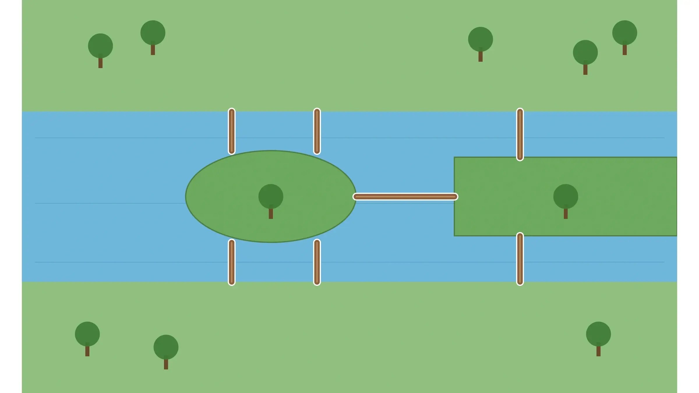
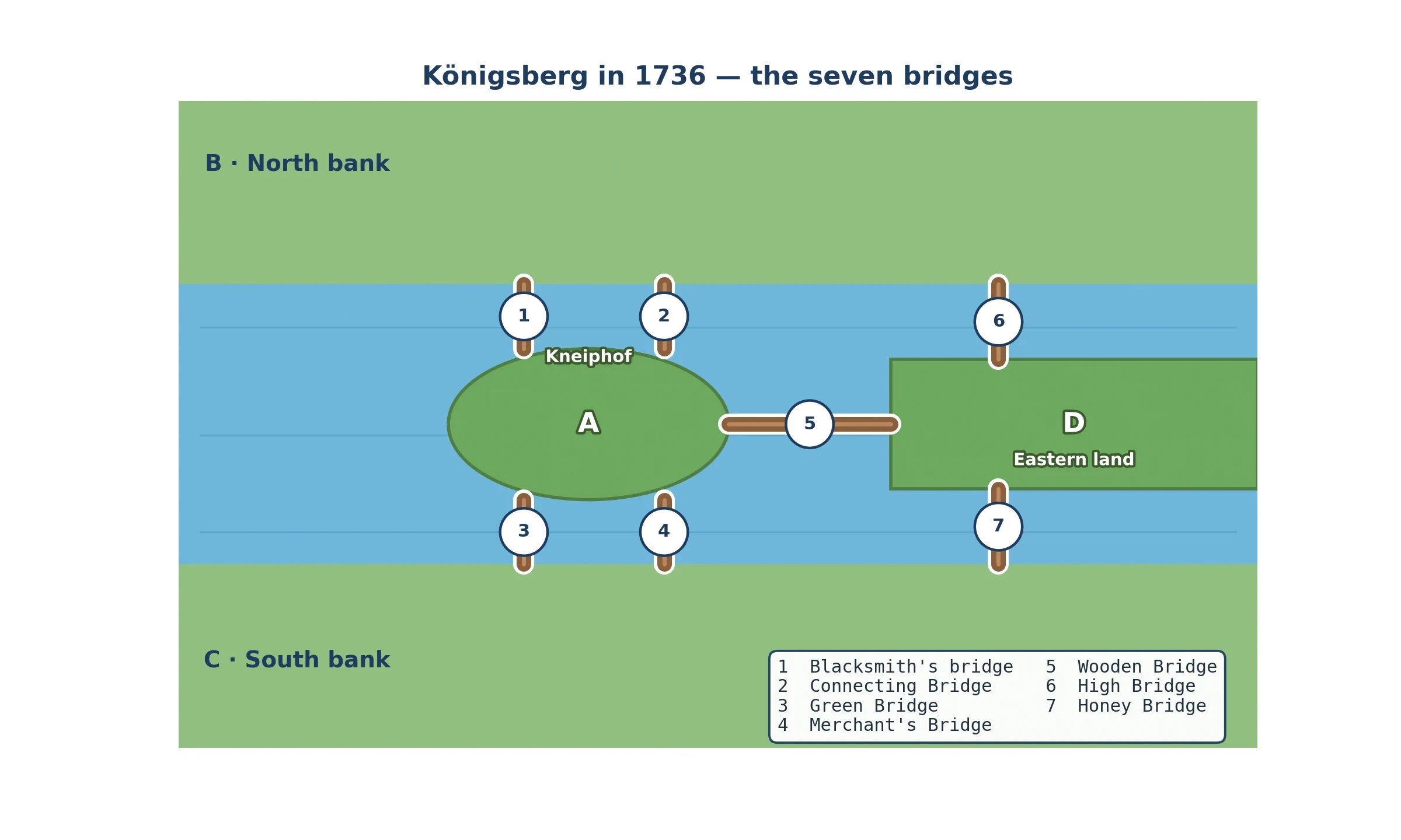
Königsberg stood where the river Pregel split around two islands. The city is Kaliningrad today, in Russia, but in 1736 it was a Prussian port. Four pieces of land were involved: the larger island of Kneiphof, the north bank, the south bank, and the eastern land mass where the river forked. The puzzle asked for a single walk that used every bridge exactly once. People failed in a way that suggested no walk existed at all.
A puzzle the whole town tried
The puzzle belonged to everyone: no mathematics needed, only a pair of shoes and an afternoon. People tried routes the way you try a maze. Some routes got tantalisingly close: a walker might cross six bridges without repeating one, then find the seventh on the wrong side of the river. Each near miss suggested the walk was possible, so people kept trying. What nobody could see was that the near misses were the shape of the answer, hiding in plain sight.
I know the feeling of those near misses, because I tried the puzzle myself long before I understood it. I drew a rough map of Königsberg and spent an evening tracing routes with my finger. I started on Kneiphof and tried route after route. Every attempt ended the same way: one bridge left, standing on the wrong piece of land. Then came a stranger feeling: the suspicion that the puzzle was not hard but impossible. That suspicion was the beginning of graph theory in my own head.
Seven bridges, four pieces of land
The seven bridges had names: the Blacksmith's bridge, the Connecting Bridge, the Green Bridge, the Merchant's Bridge, the Wooden Bridge, the High Bridge, and the Honey Bridge. Seven bridges, four land masses, and one rule: cross each bridge exactly once. Look at the map in Figure 1 and notice what the puzzle leaves out: it does not matter how long any bridge is, or how wide the river runs. All that matters is which pieces of land each bridge joins. That is the first great move of graph theory: throw away the geography and keep the connections. Once you see the town that way, the puzzle becomes a question about counting, and counting is something mathematics can settle for good.
The man who stopped trying and started thinking
The puzzle reached Leonhard Euler, the Swiss mathematician then working at the Academy of Sciences in St Petersburg. Euler was born on 15 April 1707 in Basel, and by 1736 he was among the most productive mathematicians alive. He presented his solution to the St Petersburg Academy on 26 August 1735, and it was published in 1741. The paper is often dated 1736, the year of the volume of the Commentarii in which it appeared; Euler presented it on 26 August 1735, and it was not actually printed until 1741. The full story is set out in the Mathematical Association of America's account of Euler's solution to the Königsberg bridge problem.
Euler's first reaction is the most human part of the story. He thought the problem trivial, and wrote to Carl Leonhard Gottlieb Ehler, the mayor of Danzig, who had written to him about the puzzle.
"Thus you see, most noble Sir, how this type of solution bears little relationship to mathematics, and I do not understand why you expect a mathematician to produce it, rather than anyone else, for the solution is based on reason alone, and its discovery does not depend on any mathematical principle. …" — Leonhard Euler, letter to Carl Leonhard Gottlieb Ehler, 3 April 1736.
Euler was wrong about one thing in that letter and right about the thing that mattered. He was wrong that the solution bore little relationship to mathematics: it became the first theorem of a new branch of mathematics. He was right that it was based on reason alone, since no known principle covered it. Euler threw away the map and kept four land masses, seven links, and a count of how many links touched each one. That count decided the puzzle. What did Euler throw away, and what did he keep? That question drives the rest of this article.
2. What Is Graph Theory?
Graph theory is the study of dots joined by lines, and of everything that follows from that picture. A dot stands for a thing: a place, a person, a page, a molecule. A line stands for a connection between two of those things: a bridge, a friendship, a link, a bond. Graph theory asks what you can learn from the pattern of connections alone, ignoring almost everything else about the things themselves. That is the whole of graph theory in one paragraph, and it is also the answer to the question this article keeps returning to: what did Euler keep when he threw the map away? He kept the dots and the lines.
Dots, lines, and nothing else
A graph, in graph theory, is a set of vertices joined by edges, usually written as G = (V, E), where V is the set of vertices and E is the set of edges. The words sound formal, but the idea is plain. A vertex is a dot. An edge is a line joining two dots. That is all a graph is, and the spareness is the point. By refusing to say what the dots are, graph theory can say something about all of them. The same reasoning that settles the Königsberg bridges also settles questions about road networks, friendships, and computer chips, because all of them are dots and lines underneath.
The power of the picture comes from what it leaves out. A graph of Königsberg does not record how wide the river is, or how long each bridge runs. It records only which land masses each bridge joins. Once the irrelevant detail is gone, the pattern stands out clearly enough to count, to test, and to prove things about. Graph theory is the habit of asking which details change the answer, and throwing the rest away.
The art of throwing away the right details
Every good abstraction is a gamble. Throw away too little, and the problem stays tangled. Throw away too much, and the answer stops meaning anything. Euler won his gamble because the bridges puzzle depended on connections and nothing else. Graph theory makes that gamble over and over, and its skill lies in knowing what to keep.
The everyday version of this move hangs in every underground station. A tube map is not a map of the city. It gets the distances wrong, bends the lines, and puts stations in the wrong places. What it gets right is the connections: which line serves which station, and where you change from one line to another. That is all a traveller needs. The tube map is a graph, and it works because somebody threw away the right details.
What counts as a graph, and what does not
Two confusions are worth clearing up early, because they trip up nearly everyone who meets graph theory for the first time. The first is the word graph itself. In school, a graph usually means a chart: a curve drawn on axes, showing how one quantity changes with another. That is not what graph theory studies. A graph in graph theory is not a picture of a function. It is a picture of relationships, a set of dots and the lines between them. The two uses share a history, but they are different objects, and mixing them up causes real confusion.
The second confusion is subtler. A graph is not a picture of a thing. It is a picture of how things relate. A drawing of a bridge is a picture of a bridge; a graph of Königsberg is a picture of which land masses the bridges join. That is why the same graph can describe a town, a social network, and a molecule. When you learn to see patterns of relationships instead of pictures of things, you are thinking the way graph theory thinks.
3. The Vocabulary of Dots and Lines
Every subject needs words for its basic objects, and graph theory needs very few. A handful of terms covers nearly everything graph theory talks about. Learn these words now, and the rest of the article will read like plain English, because the theorems of graph theory are mostly short sentences about dots, lines, and the numbers that describe them. The words are vertex, edge, degree, path, cycle, and a few kinds of graph.
Vertices and edges
A vertex is a dot, and an edge is a line joining two dots. In Königsberg the vertices were the four land masses and the edges were the seven bridges. In a social network the vertices are people and the edges are friendships. In the web graph the vertices are pages and the edges are links. The word graph itself is younger than graph theory: James Joseph Sylvester introduced it in a paper in Nature in 1878, more than a century after Euler solved the bridges puzzle. The name stuck because it fits. A graph is a drawing, and the drawing is the reasoning.
Degree: how connected is a dot?
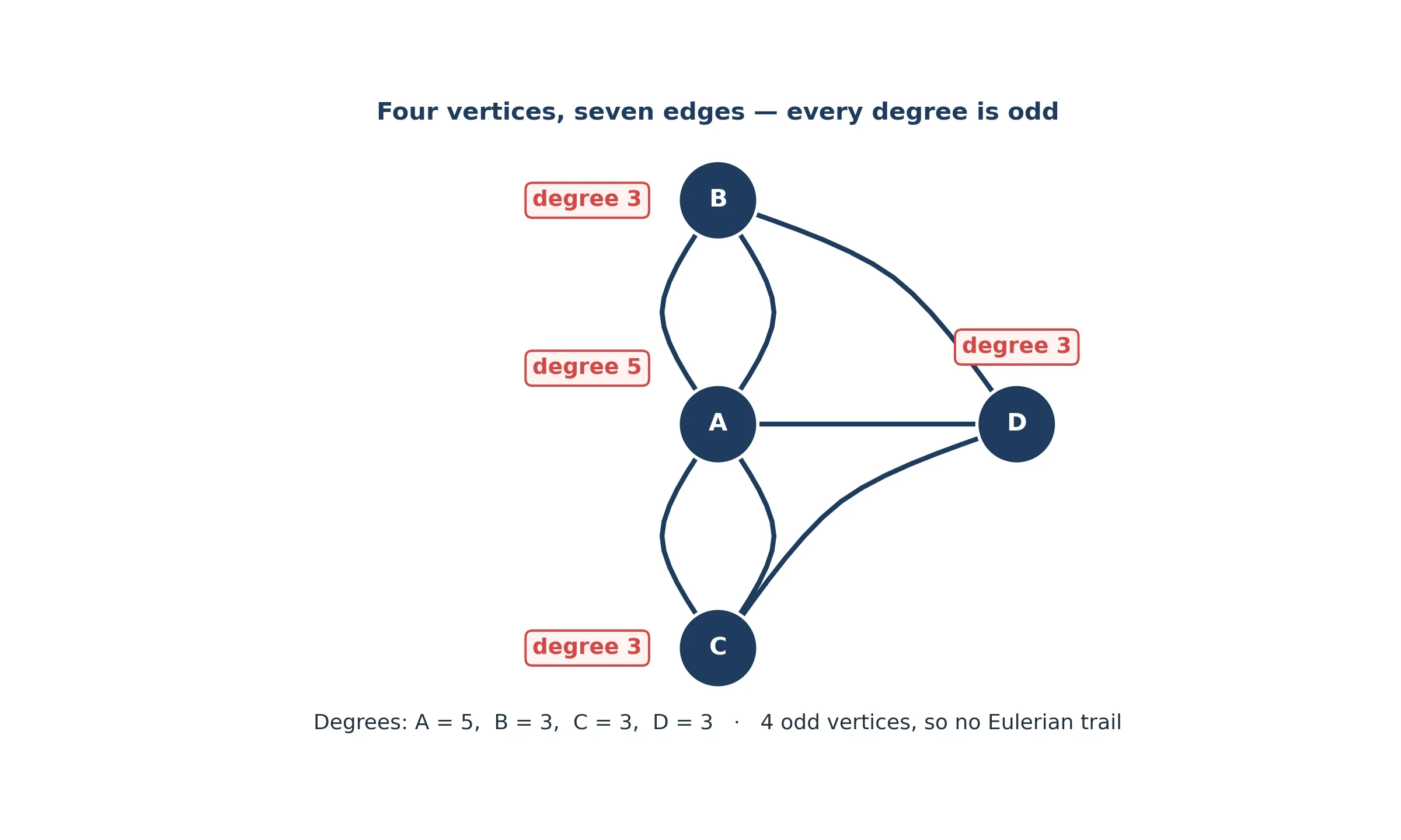
The degree of a vertex is the number of edges touching it. Kneiphof island had degree 5 in 1736, because five bridges touched it. A person with forty friends in a social network has degree 40. Degree is the first number graph theory reaches for, because it is the simplest summary of a vertex's place in the network, and a surprising amount follows from counting degrees alone. Euler settled Königsberg by counting four degrees.
Counting degrees has a payoff: the total always comes out even, and that single fact decides the Königsberg puzzle, as the next section shows.
Paths, cycles, and connectedness
A path is a route through a graph: a sequence of vertices joined by edges, with no edge used twice. A cycle is a path that returns to where it started, closing a loop. A graph is connected when there is a path between every pair of vertices, so that you can travel from any dot to any other dot along the edges. These three words carry most of graph theory's geography. A walk across Königsberg is a path. A walk that returns home is a cycle. A town whose bridges join all four land masses into one piece is a connected graph, and Königsberg was one.
A path that uses every edge exactly once is an Eulerian trail, and a path that visits every vertex exactly once is a Hamiltonian path. The two sound like twins, but they behave nothing alike, and sections 5 and 6 take that difference up in full. For now, keep the two ideas apart: edges once, or vertices once. Confusing them is the most common beginner's mistake.
Directed, weighted, and complete graphs
Real networks often need one extra idea. A directed graph gives its edges a direction, like one-way streets: the edge from A to B is not the same as the edge from B to A. A web link is directed, because a page can link to another without being linked back. A weighted graph gives its edges numbers, like distances or travel times, so that some routes cost more than others. Direction matters when you ask who can reach whom. Weight matters when you ask for the cheapest or fastest route.
A complete graph goes the other way and adds every possible edge: every vertex joined to every other vertex. The complete graph on n vertices is written K_n, and it has n times n minus 1, divided by 2, edges. K_5 has 5 times 4 divided by 2, which is 10 edges, and K_6 has 6 times 5 divided by 2, which is 15 edges. Complete graphs are the richest possible networks, and they turn up whenever a problem asks about groups where everybody knows everybody, which is why they star in the party puzzle of section 15.
4. Euler's Test: The Odd-Degree Rule
Euler's solution to the Königsberg bridge problem is one of the shortest great proofs in graph theory: it uses nothing but counting. He kept four land masses, seven bridges, and one number for each land mass: how many bridges touched it. That number is the degree, and the degrees of Königsberg decide the puzzle completely. Once you see how the counting works, you will know, before you set out, that no route exists, and you will know why.
Counting bridges at each land mass
Draw Königsberg as a graph: four dots for the land masses, seven lines for the bridges. Now count the lines touching each dot. Kneiphof island has degree 5, because five bridges touch it. The north bank has degree 3, the south bank has degree 3, and the eastern land mass has degree 3. Add them up: 5 plus 3 plus 3 plus 3 makes 14, which is twice the number of bridges. The striking fact is that all four degrees are odd, and that single fact kills the walk.
The handshaking lemma
The counting obeys a rule so simple it feels like a trick. Add up the degrees of all the vertices in any graph, and the total is always twice the number of edges, because every edge touches two vertices and contributes one to the count at each end. This is the handshaking lemma, named for the party where every handshake involves two hands. It has a sharp consequence: the number of vertices with odd degree is always even, since odd numbers must pair up to make an even total. Königsberg has four odd-degree vertices, and the number four is exactly the problem.
Why an odd vertex breaks the walk
Think about what happens in the middle of a walk. Every time you arrive at a land mass, you arrive on one bridge, and every time you leave, you leave on another. Arrival and departure come in pairs, so a land mass you pass through uses up its bridges two at a time. A land mass with an even number of bridges can be passed through cleanly until its bridges run out. A land mass with an odd number cannot: sooner or later you arrive on its last unused bridge and find no unused bridge left to leave on. Only two places escape the pairing: the start, with one extra departure, and the finish, with one extra arrival. A walk that uses every bridge exactly once can therefore have at most two land masses with odd degree. Königsberg has four, and a walk has only two ends. You cannot fit four odd vertices into two ends, and no choice of route can fix it, because the argument never mentions routes.
The rule, stated properly
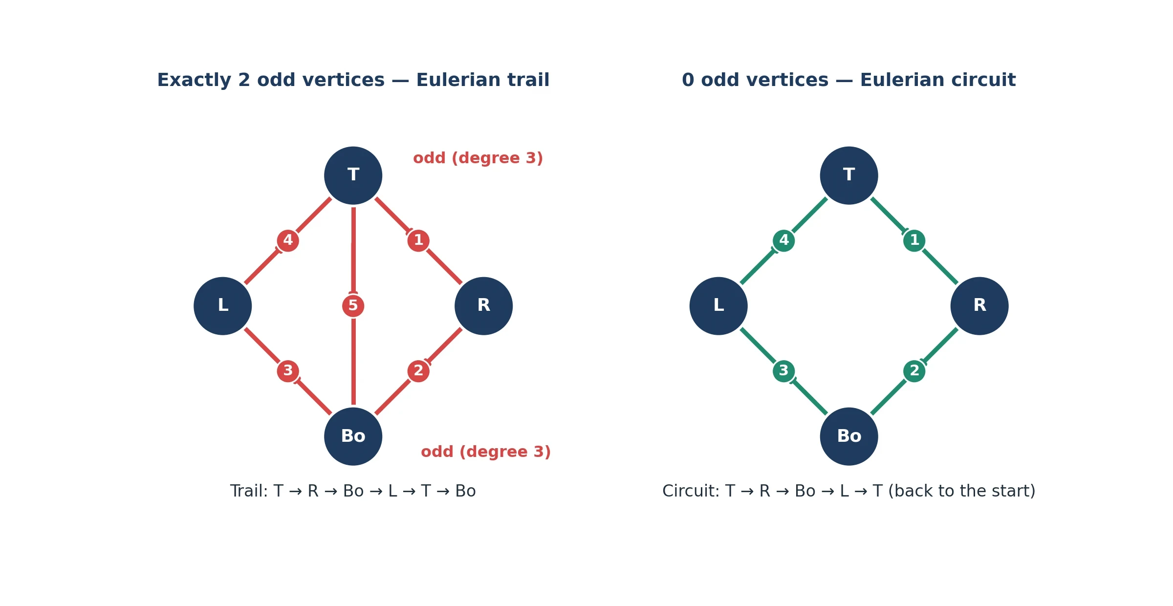
Euler's theorem, the first great result of graph theory, covers every connected graph. If every vertex has even degree, the graph has an Eulerian circuit: a trail that uses every edge exactly once and returns to its start. If exactly two vertices have odd degree, the graph has an Eulerian trail that is not a circuit: it starts at one odd vertex and ends at the other. If any other number of vertices has odd degree, four or six or eight, then no Eulerian trail exists at all. Königsberg has four odd vertices, so it falls in the third case. No trail, no circuit, no walk. The theorem is a test: count the odd degrees, and the answer is immediate.
I learned this test the slow way, on paper. I drew the four dots and the seven lines, and wrote the degree beside each dot: 5, 3, 3, 3. I stared at the four odd numbers, and then I tried to pair them off the way a walk would have to. The start could absorb one odd vertex. The end could absorb one more. Two were left over with nowhere to go, and suddenly the whole puzzle collapsed into that leftover pair. I remember the click of it, a problem going from mysterious to obvious in a single breath. I had spent an evening tracing routes that could never work, and the answer had sat in four small numbers all along.
The same counting reaches far beyond Königsberg: whenever a problem asks whether a network can be crossed or traced without repetition, the first step is to count odd degrees. The test works on road networks, on wiring diagrams, and on graphs so large no human could draw them. It even reaches graphs that go on forever, though the infinite case needs extra conditions, and the puzzles of infinity belong with Cantor and Hilbert's Hotel in our article on infinity. For finite graphs, the rule is complete: count the odds, and you know.
5. Eulerian Paths: Using Every Edge Once
In graph theory, an Eulerian trail uses every edge of a graph exactly once. An Eulerian circuit is an Eulerian trail that starts and ends at the same vertex. The difference between the two is one vertex: the finish. In a circuit, the finish is the start, so every vertex is passed through in pairs and every degree must be even. In a trail that is not a circuit, the start and finish are different vertices, and those two are allowed to be odd, because the start has one unpaired departure and the finish has one unpaired arrival. The exact statements, with worked examples, are set out in the LibreTexts chapter on Eulerian and Hamiltonian graphs.
Trails, circuits, and the difference that matters
The pen-and-paper version is familiar to every child who has tried to draw a shape without lifting the pen. A house, a star, an envelope: some can be drawn in one stroke and some cannot, and the test is the same count. Count the points where an odd number of lines meet. If there are none, you can draw the shape in one stroke and end where you began. If there are exactly two, you can draw it in one stroke from one odd point to the other. If there are four or more, no single stroke will do it. Children discover this by trial. Euler proved it by counting.
Hierholzer's proof, 1873
Euler proved that an Eulerian circuit requires all even degrees, and stated without proof that even degrees were enough. The missing half came more than a century later, from Carl Hierholzer. He presented his work to a circle of fellow mathematicians shortly before his early death in 1871, at the age of thirty. A colleague arranged its publication after his death, and the paper appeared in 1873 in Mathematische Annalen. The year is sometimes given wrongly as 1871, the year Hierholzer died, not the year his proof was published. His construction is still the method computers use today: follow unused edges until you close a cycle, then splice in further cycles from vertices with unused edges, repeating until none remain. Because the degrees are even, you never get stuck except at a closed cycle. The proof works by building, and it turns Euler's test into a recipe.
Königsberg today
Königsberg is Kaliningrad now, and its bridges are not those Euler knew. Two of the seven bridges were destroyed in the Second World War, and the city rebuilt its crossings differently. Today only five bridges join the same four land masses. The change is small, but it changes the arithmetic completely. With five bridges, the degrees add to 10, twice the number of edges, and the degree set is 3, 2, 2, 3: exactly two land masses have odd degree. Euler's theorem, the founding test of graph theory, now gives a different answer. An Eulerian trail exists, because exactly two vertices are odd, but an Eulerian circuit does not, because a circuit needs zero odd vertices. So the walk that defeated Königsberg for centuries is possible today, with one condition: start at one of the two odd-degree land masses and finish at the other. Start anywhere else, and the walk fails.
Where Eulerian paths earn their keep
Eulerian trails are the working mathematics of any job that must cover every street, pipe, or wire exactly once. A snowplough clearing every street in a neighbourhood wants an Eulerian trail through the street graph, so that it never reploughs a cleared street. A street sweeper wants the same. A postman delivering along every road in a district wants a route that covers each road once. The test comes first: count the odd-degree junctions, and you know whether a perfect route exists before you plan anything. The most surprising application sits inside DNA-reading machines. Sequencing a genome produces millions of short fragments, and reassembling them means finding a trail that uses every fragment once. The graph is enormous, but the same test applies, and the counting makes the reassembly fast enough to be practical.
6. Hamiltonian Paths: Visiting Every Vertex Once
Euler asked for a walk that uses every edge once. More than a century later, William Rowan Hamilton asked a question that sounds almost the same and behaves nothing like it: a walk that visits every vertex once. Hamilton turned his question into a game, the Icosian Game, exhibited in 1857 and sold from 1859. The board was a dodecahedron, a solid with twenty corners, and the challenge was to find a route that visited every corner exactly once and returned to the start. It was a parlour game, but the puzzle underneath it has resisted every attempt at a simple answer ever since.
Hamilton's Icosian Game, 1857
The Icosian Game came with a wooden board, pegs, and a string, and the player had to lay the string along the edges of the dodecahedron so that it passed through all twenty corners exactly once. Hamilton, the Irish mathematician who had already revolutionised physics with his work on mechanics, marketed the game as a puzzle for the drawing room. It was a commercial failure. Finding a route through all twenty corners is easy enough on a dodecahedron, but Hamilton's question in general, for any graph, has no neat answer, and the game was the first public face of a problem that would become one of the central mysteries of computer science.
Edges versus vertices: why the twin problem is nothing alike
Most people assume the Hamiltonian problem is Euler's problem with the words swapped: edges once, vertices once, same puzzle. That assumption is wrong, and the difference is one of the sharpest lessons in graph theory. Euler has a test. Count the odd degrees and you know immediately whether a trail exists, for any graph, however large. Hamilton has no test. There is no counting trick, no degree rule, no simple condition that tells you whether a Hamiltonian path exists. Deciding whether a Hamiltonian cycle exists is NP-complete, which means that no fast general method is known, and that the best known methods must in the worst case try something close to every possible route. The two problems look like twins and behave like strangers.
The reason is that edges are local and vertices are global. Euler's test works because the degree of a vertex is a local fact, and the handshaking lemma ties local facts into a global answer. A Hamiltonian path is a global demand: the route must visit every vertex, and a choice made at one end of the graph can ruin the route at the other end. There is no local count that captures that. You can have a graph where every vertex has high degree and still no Hamiltonian cycle exists, because the graph is pinched in the middle, with a narrow bridge that the route cannot cross twice. Degree counts cannot see the pinch.
Dirac 1952 and Ore 1960: guarantees that sometimes work
Mathematicians have found conditions that guarantee a Hamiltonian cycle, and two are worth stating exactly, because they show what a partial answer looks like. Dirac's theorem, proved in 1952, says that a simple graph with n vertices, where n is at least 3, and every vertex has degree at least n divided by 2, must have a Hamiltonian cycle. Ore's theorem, proved in 1960, says that a simple graph with n vertices, where n is at least 3, and the degrees of every pair of non-adjacent vertices add to at least n, must have a Hamiltonian cycle. Both are sufficient conditions, not necessary ones: a graph can have a Hamiltonian cycle while failing both. The theorems catch many graphs and miss many others, and that gap is the whole difficulty. A test that only sometimes says yes is not a test at all.
The travelling salesman
The travelling salesman problem is the Hamiltonian problem wearing work clothes. A salesman must visit a set of cities once each and return home by the shortest possible route. Every route is a Hamiltonian cycle, and the number of possible routes grows with shocking speed. The number of distinct Hamiltonian cycles in a complete graph on n vertices is n minus 1 factorial, divided by 2. For 5 cities there are 12 possible routes. For 10 cities there are 181,440. For 20 cities there are more than sixty thousand trillion. That factorial growth is why delivery companies, airlines, and chip designers need clever algorithms rather than brute force, and why counting routes is a problem for probability as much as for graph theory, a connection our article on what probability is takes up in full.
| Eulerian path | Hamiltonian path | |
|---|---|---|
| Visits | Every edge exactly once | Every vertex exactly once |
| Test | Count odd degrees: 0 gives a circuit, 2 gives a trail | No simple test exists |
| Difficulty | Easy to decide; Hierholzer's algorithm finds the trail | NP-complete; no fast general algorithm is known |
| Home puzzle | The Königsberg bridges | The Icosian Game |
Table 1: Euler versus Hamilton, side by side. One problem has a test and the other does not, and that difference shapes everything that follows.
7. Trees: The Graphs With No Shortcuts
In graph theory, a tree is the simplest kind of connected graph. It is a graph with no cycles: no route that leaves a vertex and returns to it without reusing an edge. That restriction explains why trees turn up everywhere, from the folder system on your computer to the cables under a city street. Between any two vertices there is exactly one route, and that uniqueness is what makes trees easy to work with and easy to count.
What makes a tree a tree
A tree is a connected graph with no cycles. Connected means you can travel from any vertex to any other vertex along the edges. No cycles means there is no closed loop anywhere. Put the two together and you get the property that defines trees: exactly one route between any two vertices, since two different routes would form a cycle. That uniqueness is why trees are the natural shape for anything that must branch without ever rejoining: a family tree, a company org chart, a folder system where each folder sits inside exactly one parent.
A tree on n vertices has n - 1 edges
Count the edges of a tree and a pattern appears at once. A tree on 4 vertices has exactly 3 edges, on 5 vertices 4 edges, and on 10 vertices 9 edges. The rule is that a tree on n vertices has exactly n minus 1 edges, no more and no fewer. Start with one vertex and no edges. Each new vertex needs exactly one edge to keep the graph connected, and a second edge would create a cycle. So each new vertex costs one edge, and n vertices cost n minus 1 edges. Adding an edge to a tree creates exactly one cycle, because the two vertices it joins were already connected by exactly one route, and the new edge closes that route into a loop.
Cayley's counting surprise
How many different trees can you draw on the same set of labelled vertices? The answer, found by Arthur Cayley in 1889, is a surprise: the number of labelled trees on n vertices is n to the power n minus 2. For 4 labelled vertices there are 16 trees, for 5 labels 125, for 6 labels 1,296, and for 10 labels 100,000,000. The numbers explode, and the formula is exact, not an estimate. Cayley stated it in his paper "A Theorem on Trees", and the first proof by direct counting came from Heinz Prüfer in 1918, nearly thirty years later, using a clever code that turns each tree into a unique sequence of labels and back again. The surprise is that so many different trees can live on the same handful of dots.
Spanning trees and the cheapest network
A spanning tree is a subgraph that is a tree and contains every vertex of the graph. Given any connected network, you can strip away edges until only a spanning tree remains, and the result still connects everything, with no wasted edge. That makes spanning trees the answer to a practical question: how do you connect a set of places at the lowest cost? Laying cable, fibre, or road costs money per edge, so the cheapest network that connects everything is the minimum spanning tree. Kirchhoff counted spanning trees with a determinant as early as 1847. Boruvka solved the minimum spanning tree problem in 1926 for a real power network in Moravia, finding the cheapest way to wire a region for electricity. Kruskal's and Prim's algorithms came later, and they run on the same idea: keep adding the cheapest edge that does not create a cycle, until everything is connected.
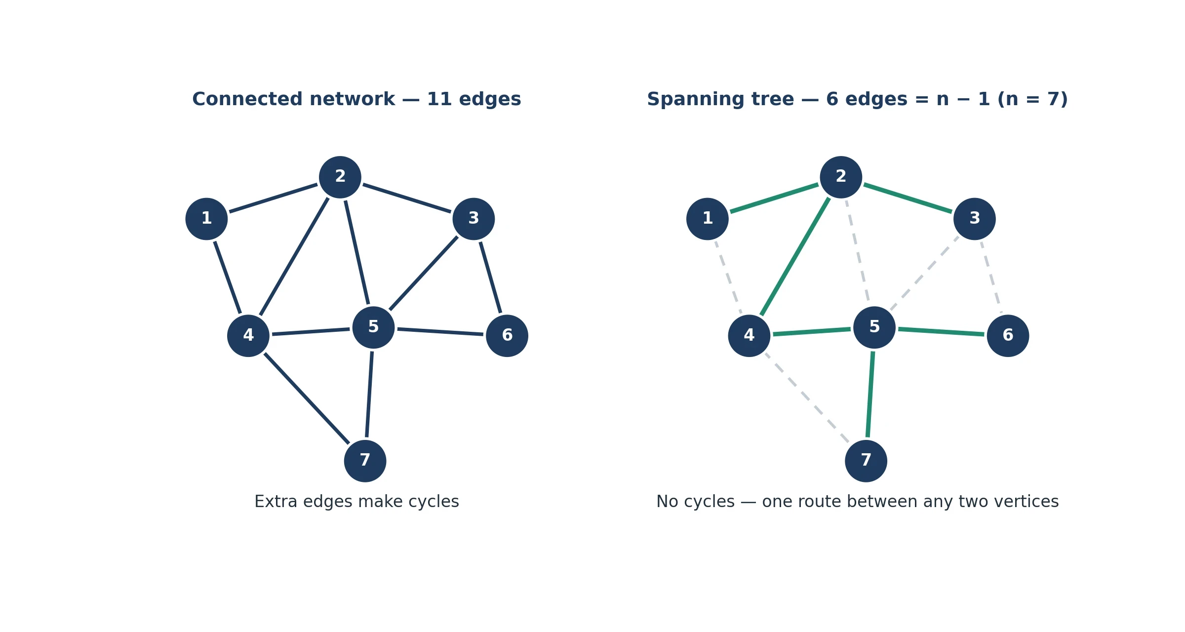
Phylogenetic trees are trees in exactly this sense, and the family tree of life is one of the largest trees science has ever drawn, as our article on the tree of life shows. A tree is a promise: one route between any two points, no loops, no waste, and a count you can do on your fingers.
8. Euler's Formula: V - E + F = 2
Euler's second great gift to graph theory is a formula so short you can write it on your hand: V minus E plus F equals 2. V counts the vertices, E counts the edges, and F counts the faces, the regions into which the edges divide the surface. For any connected planar graph, the three numbers always combine to 2.
Counting corners, edges, and faces
Euler first wrote the formula in a letter to Christian Goldbach, dated 14 November 1750. He stated it in print in 1758, in the form that relates the corners, edges, and faces of a polyhedron: the number of vertices minus the number of edges plus the number of faces always equals 2. The first rigorous proof came from Adrien-Marie Legendre in 1794, more than forty years after Euler stated it. Euler saw the pattern clearly, but a proof that left no hole took another generation.
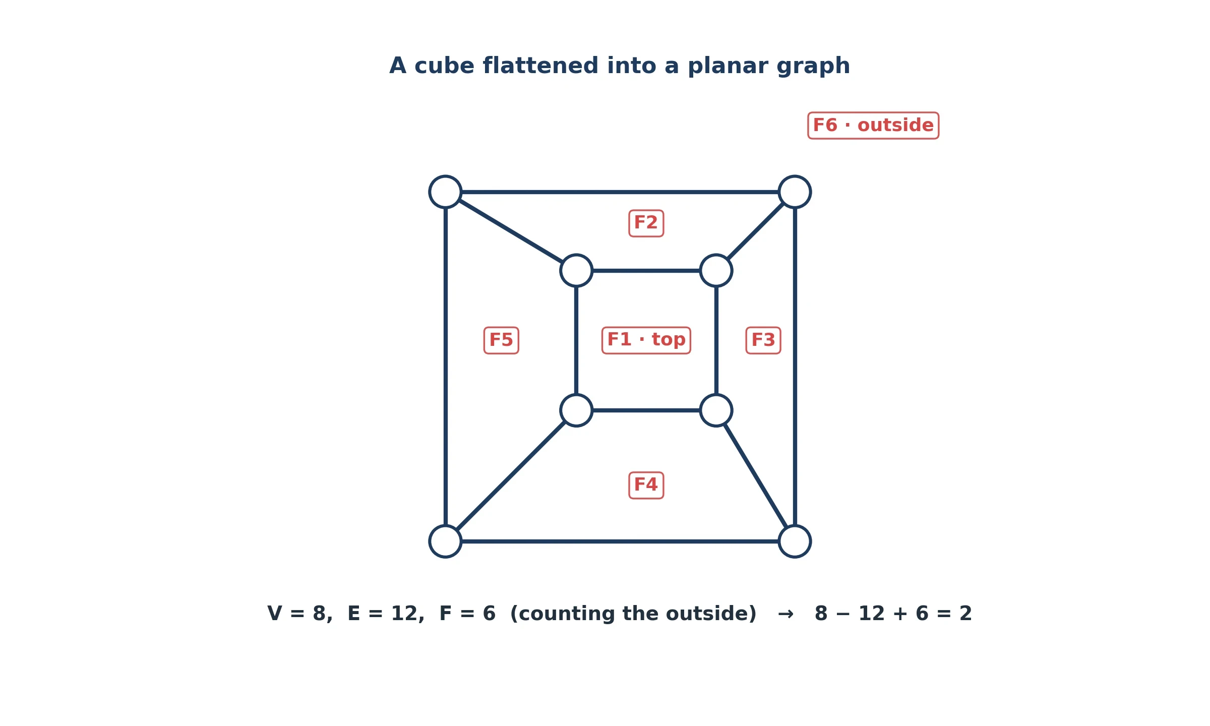
A face is a region bounded by edges, and the definition has one surprising feature: the outside counts too. Draw a triangle on a page. It has 3 vertices and 3 edges, and it divides the page into two faces: the inside of the triangle and the outside, the rest of the page stretching away. The formula gives 3 minus 3 plus 2, which is 2. Forget the outside face and the count fails.
Five solids, one answer
In graph theory, the formula earns its reputation on the five Platonic solids, the perfectly regular solids the Greeks knew. Each one gives the same answer, 2, and the arithmetic is worth doing in full. The tetrahedron has 4 vertices, 6 edges, and 4 faces: 4 minus 6 plus 4 is 2. The cube has 8 vertices, 12 edges, and 6 faces: 8 minus 12 plus 6 is 2. The octahedron has 6 vertices, 12 edges, and 8 faces: 6 minus 12 plus 8 is 2. The dodecahedron has 20 vertices, 30 edges, and 12 faces: 20 minus 30 plus 12 is 2. The icosahedron has 12 vertices, 30 edges, and 20 faces: 12 minus 30 plus 20 is 2. Five solids, five different sets of numbers, one answer every time.
The solids themselves belong to geometry, and our article on Euclidean geometry tells that story. This article owns the formula, which is a fact of graph theory about graphs drawn on a surface. Flatten any solid onto a page, count its corners, edges, and regions, and the same arithmetic holds. The formula cares only that the graph is connected and drawn without crossings, and that every region, including the outside, is counted.
The outside counts too
Flatten a cube onto the page and count again. The cube becomes a square inside a square, joined at the corners, with 8 vertices and 12 edges, just like the solid. The faces are the six regions of the drawing: the four side faces, the top face in the middle, and the outside region, which is the bottom face of the cube, stretched around the whole picture. Count all six and the formula gives 8 minus 12 plus 6, which is 2. Leave the outside out and you get 1. The outside is a face like any other, and the formula only works when every region is counted.
You can check the formula at home with a football. A standard football is a truncated icosahedron, a ball sewn from pentagons and hexagons, and it obeys the same arithmetic as the five perfect solids. Count its corners, its seams, and its panels, and the three numbers will combine to 2. It is a satisfying check, because it turns a formula about abstract graphs into something you can hold in your hands.
| Solid | Vertices (V) | Edges (E) | Faces (F) | V - E + F |
|---|---|---|---|---|
| Tetrahedron | 4 | 6 | 4 | 2 |
| Cube | 8 | 12 | 6 | 2 |
| Octahedron | 6 | 12 | 8 | 2 |
| Dodecahedron | 20 | 30 | 12 | 2 |
| Icosahedron | 12 | 30 | 20 | 2 |
Table 2: The five Platonic solids. Different vertices, edges, and faces every time, and the same answer, 2, in the last column.
9. Planar Graphs and the Two Forbidden Patterns
In graph theory, a planar graph is a graph that can be drawn on a flat page with no edge crossings. The definition sounds modest, but it decides real questions. A circuit board is a planar graph problem: the wires are edges, the components are vertices, and every crossing costs a layer of board or a redesign. A chip designer wants to know whether a circuit can be laid out flat, and graph theory answers with a test naming exactly two forbidden patterns.
Drawing without crossings
Planarity is a property of the graph, not of any one drawing. A graph is planar when some drawing of it has no crossings, even if the first drawing you try is a tangle. Untangling earphone cables is the everyday version: some tangles can be undone by patient pulling, and some cannot be undone without lifting a wire over another. The same is true of graphs. A planar graph can always be untangled. A non-planar graph cannot, and the reason is always one of two patterns hiding inside it.
K5 and K3,3
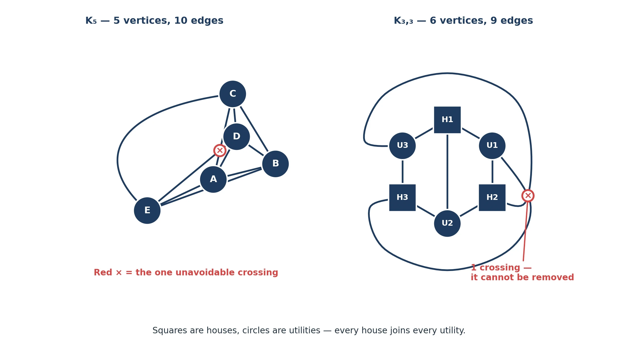
The two forbidden patterns are K_5 and K_3,3, and both fail planarity by the same kind of counting that settled Königsberg. K_5 is the complete graph on 5 vertices: every vertex joined to every other, 10 edges in total. A planar graph on 5 vertices can have at most 3 times V minus 6 edges, which is 9, and 10 is more than 9, so K_5 cannot be planar. K_3,3 is the complete bipartite graph with 3 vertices on each side, 9 edges in total. A planar bipartite graph on 6 vertices can have at most 2 times V minus 4 edges, which is 8, and 9 is more than 8, so K_3,3 cannot be planar either. Euler's formula proves the bounds: it turns a question about drawing into a question about counting.
Try drawing K_5 and you will feel the bound. Five dots, ten lines, and no matter how you arrange the dots, one crossing remains. Move a dot, reroute a line, and the crossing moves somewhere else, but it never disappears. The same happens with K_3,3. The crossing is not a failure of imagination. It is arithmetic: there are simply too many edges for the faces available. Figure 6 shows both graphs with one unavoidable crossing each. The crossing is not a mistake in the drawing. It is the proof.
Kuratowski 1930 and Wagner 1937
The full test for planarity is Kuratowski's theorem, published in 1930. It says that a finite graph is planar exactly when it contains no subdivision of K_5 or K_3,3. A subdivision is a stretched copy: take K_5 or K_3,3, insert extra vertices along the edges, and you still have the same forbidden pattern, only longer. Any graph that hides such a copy is non-planar, and any non-planar graph hides one. Wagner proved a version of the same theorem in 1937, using minors instead of subdivisions: a graph is planar exactly when it has no K_5 or K_3,3 minor, where a minor is what you get by deleting and contracting edges and vertices. The two versions agree, and together they give planarity a complete characterisation. The MIT lecture notes on Kuratowski's planarity theorem set out the statement in full.
The three-houses-and-three-utilities puzzle
K_3,3 has a famous disguise. Three houses need gas, water, and electricity, and three utility plants stand on the other side of the road. Can you connect each house to each utility with pipes and cables that never cross? The puzzle has been handed around for a century, and the answer is no. The houses and the utilities form K_3,3: three vertices on one side, three on the other, nine edges, and the planar bound says eight is the most a flat drawing allows. The ninth connection must cross one of the others, and no rearrangement will change that. The puzzle feels like a challenge to your ingenuity, and it is really a test of your willingness to accept a counting argument.
10. Colouring Maps: The Four Colour Theorem
How many colours does a map need? Four sounds too small to be true. Look at any atlas and you will see maps coloured with far more than four colours, because mapmakers like variety. But the claim of the four colour theorem is narrower and stronger: any map can be coloured with four colours so that no two regions sharing a border get the same colour. The theorem took 124 years to prove and broke two published proofs along the way, and its final proof needed a computer.
A mapmaker's hunch
The story starts in October 1852, with Francis Guthrie colouring a map of English counties. Guthrie noticed that he never needed a fifth colour, and wondered whether four would always be enough. His brother Frederick put the question to Augustus De Morgan, who wrote about it to William Rowan Hamilton on 23 October 1852. Guthrie's hunch was a guess, not a theorem, and nobody could prove it. The question sat there, simple to state and impossible to settle.
Eleven years of a false proof
In 1879, Alfred Kempe published a proof that four colours always suffice, and the mathematical world accepted it. For eleven years, the four colour theorem was considered proved. Then, in 1890, Percy Heawood found the flaw. Kempe's argument worked for most maps, but it broke on a particular kind of region, and no repair could save it. Heawood demolished the proof, and in the same paper proved that five colours always suffice. Five was easy. Four was the hard part. In 1880, Peter Guthrie Tait published a second proof, and it stood until Julius Petersen refuted it in 1891. Two proofs, two demolitions.
1976: the computer enters the proof
The answer came from Kenneth Appel and Wolfgang Haken, at the University of Illinois. They announced their proof on 21 June 1976 and published it in 1977. Their method was to reduce the problem to a list of configurations, each small enough for a computer to check, and then to show that every map contains at least one configuration from the list. The proof checked an unavoidable set of nearly two thousand configurations — 1,482 in the published version. The computer work took 1,200 hours on an IBM 360, and the result was the first major theorem proved with essential computer assistance. No human could check 1,482 configurations by hand. The computer did the checking, and the mathematicians did the reasoning.
The proof was controversial. Mathematicians had always believed that a proof should be something a person could read and verify, and here was a proof that no person could fully check. A small error was later found by Ulrich Schmidt, and Appel and Haken answered with a corrected account in their 1989 book. The error did not overturn the theorem, but it showed the worry was real.
A simpler proof, then a machine-checked one
In 1997, Robertson, Sanders, Seymour, and Thomas published a simpler proof using 633 configurations, though it still needed a computer for the checking. The answer to the worry came in 2005, when Georges Gonthier and Benjamin Werner formally verified the four colour theorem in the Coq proof assistant. A proof assistant checks every step against the rules of logic, and accepts nothing on trust. The formal proof ran to about 60,000 lines, and Gonthier's account appeared in the Notices of the American Mathematical Society in 2008. Between them, the three proofs trace the arc of graph theory: a proof that needed a machine, a simpler one, and a machine-checked one.
What counts as a proof?
The four colour theorem forced graph theory to ask a question it had never asked seriously before: what counts as a proof? A proof is an argument that convinces the experts, and for most of history that meant an argument a person could read from start to finish. The computer proofs broke that pattern. They convinced the experts, but no expert could read them in full. The question is about trust and the division of labour between human reasoning and machine checking, and it is the same question science asks about evidence. Our article on the scientific method takes up how evidence earns trust in science.
Seven colours on a doughnut
The number four is special to the flat page. Change the surface and the number changes. Heawood, the same mathematician who demolished Kempe's proof, worked out what happens on a torus, a doughnut-shaped surface. Maps on a torus need at most seven colours, and seven are sometimes needed. The formula is the floor of (7 + the square root of (1 + 48 times the number of holes)) divided by 2; for a doughnut, with one hole, that is (7 + 7) / 2, which is 7. The extra colours come from the hole in the middle, which lets regions wrap around and touch in ways a flat map forbids. A map on a globe behaves like a flat page. A torus is different: the hole changes the count.
I tried colouring maps by hand once, with four crayons and a printed map of imaginary counties, hunting for the map that needed a fifth colour. I started in one corner and worked outward. Twice I painted myself into a corner, with a region surrounded by four different colours and no colour left for it. Twice I went back, changed an earlier choice, and found a way through. I never found the map that needed five colours, because Appel and Haken proved it does not exist. But the trying taught me something the theorem alone could not: four colours feel like too few, right up until you see them work.
11. Colouring Graphs: Chromatic Numbers
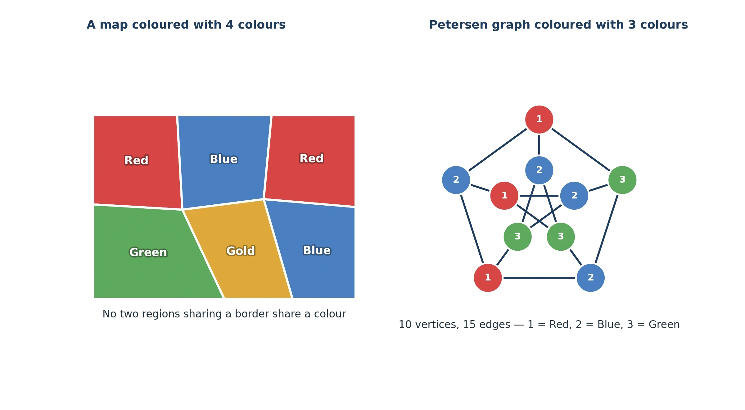
A map becomes a graph when each region becomes a vertex and each shared border becomes an edge. Two regions that share a border are adjacent vertices, and they need different colours. Two regions that meet only at a point are not adjacent, and they may share a colour. The four colour theorem, in graph language, says that every planar graph has chromatic number at most 4. The right half of Figure 7 shows the other side of graph theory: a graph that needs exactly three colours.
From maps to graphs
The translation from maps to graphs is Euler's move again. A region becomes a dot. A shared border becomes a line. The shape of the region does not matter, the length of the border does not matter, and the position of the region on the page does not matter. All that matters is which regions touch which. Once the map is a graph, the colouring problem is a question about vertices and edges. The four colour theorem is a statement about planar graphs, and that is why a theorem about maps belongs in a book about graphs.
How few colours can you get away with?
In graph theory, the chromatic number of a graph is the smallest number of colours needed to colour its vertices so that adjacent vertices always differ. It is a single number that summarises how tangled a graph is. A graph with no edges needs one colour. A single cycle needs two colours when it is even and three when it is odd, because an odd cycle cannot be coloured with two colours: the colours must alternate around the ring, and an odd ring forces two neighbours to share a colour at the join. The chromatic number is easy to define and hard to compute: for large graphs, finding it exactly can defeat fast computers.
The Petersen graph
The Petersen graph is the most famous small graph in mathematics, and the standard example of a graph that looks simple and behaves strangely. It has 10 vertices and 15 edges, every vertex has degree 3, and its chromatic number is 3: no two-colouring exists, and a three-colouring does. The graph first appeared in Kempe's 1886 paper, and Petersen constructed it in 1898. It has a Hamiltonian path, a route visiting every vertex exactly once, but no Hamiltonian cycle, a fact that can be checked by brute force. The Petersen graph is a counterexample machine: whenever a conjecture looks plausible, it is the first place to test it.
Brooks's theorem, 1941
Brooks's theorem, proved in 1941, says that for a connected graph that is neither a complete graph nor an odd cycle, the chromatic number is at most the maximum degree. A graph where every vertex has degree at most 3 can usually be coloured with 3 colours, and the Petersen graph meets the bound exactly: maximum degree 3, chromatic number 3. The exceptions are the complete graphs, which need one colour per vertex, and the odd cycles, which need 3 colours with maximum degree 2. The theorem is a guarantee of the same kind as Dirac's and Ore's: a colouring exists, but the theorem does not say how to find it. The simplest method, greedy colouring, colours vertices one at a time, always picking the first colour that does not clash with a neighbour already coloured, and never uses more than the maximum degree plus one. Greedy colouring is fast and often good, but not always best, and finding the best colouring is the hard part.
Colouring in disguise
Graph colouring wears many disguises. An exam timetable is a colouring problem: each exam is a vertex, two exams that share a student are joined by an edge, and each colour is a time slot, so that no student sits two exams at once. Radio frequencies are a colouring problem: each transmitter is a vertex, two transmitters that interfere are joined, and each colour is a frequency. Register allocation in a compiler is a colouring problem: each variable is a vertex, two variables live at the same time are joined, and each colour is a processor register. The disguises are different, but the graph is the same. Colouring as a constraint problem is a cousin of strategy, not a game, and our article on game theory shows where strategy takes over from constraint.
12. Shortest Paths: How Your Phone Finds the Way
Every time your phone finds a route, it solves a graph theory problem. Junctions are vertices, roads are edges, and travel times are weights. The question is the shortest path. The algorithm that answers it, Dijkstra's algorithm, was conceived in twenty minutes in a cafe, and it has guided travellers, packets, and delivery vans ever since.
Twenty minutes in a cafe
Edsger W. Dijkstra conceived his algorithm in 1956, in about twenty minutes, sitting in a cafe in Amsterdam. The problem was a demonstration for a new computer, the ARMAC. He first ran the algorithm on a simplified road map of 64 cities in the Netherlands. He published it in 1959 in Numerische Mathematik, in a paper titled "A note on two problems in connexion with graphs", which also re-derived the minimum spanning tree algorithm now called Prim's algorithm. Dijkstra won the ACM Turing Award in 1972, the highest honour in computer science.
The algorithm, in plain words
Dijkstra's algorithm works by settling places one at a time, always taking the nearest unsettled place first. Start at your origin with a distance of zero, and write down the travel time to each place you can reach directly. Now settle the nearest one: its shortest distance is fixed, because any other route to it would have to pass through a place at least as far away. From the settled places, look at their unsettled neighbours, update the travel times, and settle the nearest unsettled place again. Repeat until every place is settled.
The algorithm needs one condition: the weights must not be negative. A negative weight would break the settling argument, because a detour could always make a settled route cheaper afterwards.
Worked example
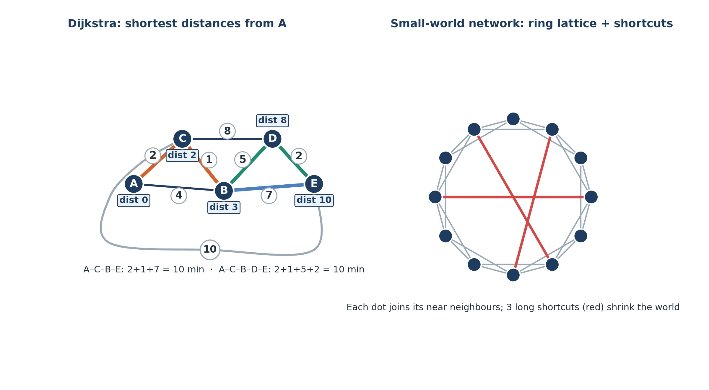
Take five places, A, B, C, D, and E, with travel times in minutes: A to B takes 4, A to C takes 2, C to B takes 1, B to D takes 5, C to D takes 8, C to E takes 10, D to E takes 2, and B to E takes 7. Start at A. The nearest place is C, at 2 minutes, so C is settled first. From C, B is reachable in 3 minutes, beating the direct road from A at 4, so B is settled next. From B, D is reachable in 8 minutes, beating the road from C at 10, so D is settled at 8. From D, E is reachable in 10. The direct road from C takes 12, and the direct road from A through B takes 11 — but the route through the settled B takes 10, tying the route through D. E is settled last at 10 minutes. The shortest distances from A are A 0, C 2, B 3, D 8, and E 10.
The shortest route from A to E takes 10 minutes, and there are two of them. One is A to C to B to E: 2 plus 1 plus 7 is 10. The other is A to C to B to D to E: 2 plus 1 plus 5 plus 2 is also 10. Both routes pass through B, and the detour through D costs exactly what the direct road from B to E saves. A navigation app would show you one of them, usually the one with fewer turns. The example is small, but the pattern is the whole algorithm.
Beyond Dijkstra
Dijkstra's algorithm is the foundation, not the finish. Modern navigation adds direction: A* search guides the search toward the destination with a guess of the remaining distance. GPS navigation adds live traffic and road closures to the same graph. The hardware that finds your position is a different story, told in our article on how GPS works. The internet uses the same idea at a larger scale: routing protocols called OSPF and IS-IS run shortest-path calculations across the network, so that each packet of data takes the cheapest route available. The packets and the protocols are a different story again, told in our article on how the internet works.
I saw the algorithm working, without knowing its name, on a drive through a city I did not know. I took a wrong turn and waited for the voice from the phone to complain. It did not complain. It paused, recalculated, and offered a new route two minutes longer than the one I had missed. I remember the calm of it: a graph with one edge removed and the shortest path found again. That is what Dijkstra's algorithm does, thousands of times a day.
13. Networks: The Small World and the Web
In graph theory, graphs become networks when the dots are people and the lines are relationships, and networks have a property that surprises everyone who measures them: they are small. The world feels large, but the network that joins it is shallow. A few steps carry you from almost anyone to almost anyone else, and that smallness shapes everything from gossip to epidemics.
Six degrees of separation
The idea of a small world is older than the experiments that tested it. In 1929, the Hungarian writer Frigyes Karinthy published a short story called "Chains", in which a character claims that any two people on Earth can be connected through five acquaintances. The phrase "six degrees of separation" came later, from John Guare's play of that name in 1990. Karinthy imagined the chain. Milgram measured it. Guare named it.
What Milgram actually found
Stanley Milgram ran the small-world experiment in 1967. Packets were sent from starters in Nebraska and Boston to a target stockbroker in Sharon, Massachusetts, who worked in Boston. Each person who received a packet was told to forward it only to a first-name acquaintance closer to the target. In the main study, analysed with Jeffrey Travers, 296 packets were sent and 64 arrived, which is 21.6 percent. The completed chains averaged 5.2 intermediaries. The Nebraska random group did worse: 100 sent, 18 arrived, mean 5.7 intermediaries. The number 5.2 describes the successful chains only, and the median was about five intermediaries: five intermediaries means six steps from starter to target, the origin of six degrees of separation.
The Watts-Strogatz model, 1998
Milgram measured the small world; Duncan Watts and Steven Strogatz explained it. In their 1998 paper in Nature, they built a model that starts with a ring lattice, where each node links to its near neighbours, and then rewires a small fraction of the edges at random into long-range shortcuts. The clustering barely changes, because most links stay local, but the average path length collapses. They tested the model on three real networks: the worm C. elegans nervous system, the western United States power grid, and the film-actor collaboration graph. All three showed high clustering and short paths. The Nature paper on collective dynamics of small-world networks has shaped the field ever since.
Measuring the whole planet's friendships
Facebook measured the small world at a scale Milgram could never have attempted. In 2011, a study of 721 million users found an average of 3.74 degrees. In 2016, a recount of 1.59 billion users found 3.57 degrees, an average distance of 4.57 friendship links, and 3.46 degrees within the United States. The numbers are averages, not maxima, and they describe Facebook's graph, not humanity. They count only the friendships on the platform. The full results are in the Meta Research post on three and a half degrees of separation.
PageRank: the web as a graph
The web is a graph, with pages as vertices and links as edges, and in 1998 Sergey Brin and Larry Page showed how to rank it. PageRank says that a page's rank depends on the number and the rank of the pages linking to it. The damping factor is usually set to 0.85, modelling a random surfer who follows links most of the time but occasionally jumps to a random page. PageRank is the probability that a person clicking links at random lands on a given page. The paper reported an index of about 24 million pages. Updating a belief from new evidence is a different tool, and it belongs in our article on Bayes' theorem.
Why the naive multiplication fails
A tempting argument says that six degrees must be true because of multiplication: if each person knows 150 people, six steps reach 150 to the power 6 people, more than enough to cover the planet. The argument is wrong, and the reason is overlap. Your 150 friends mostly know each other, and their friends are largely the same people again. The multiplication counts the same people over and over, and clustering defeats it. What saves the small world is not how many friends each person has, but the long-range weak ties: the acquaintance in another city, the colleague from a different field, the friend of a friend who lives on another continent. A few shortcuts beat millions of local links. Networks that repeat at every scale are a different idea, and they belong in our article on fractals, while the way small changes can have large effects belongs in our article on chaos theory. The right half of Figure 8 shows the shape of the answer: a ring of neighbours, with a few long shortcuts.
I once traced a chain of introductions from myself to a stranger, counting the steps as I went. A friend introduced me to a colleague, the colleague introduced me to a researcher in another city, and the researcher introduced me to the stranger, whose work I had admired from a distance. Four introductions, five people, and a conversation that would never have happened otherwise. I remember counting the steps on my fingers and feeling the smallness of the world as a physical thing. Milgram's packets did the same thing with envelopes; mine did it with handshakes.
14. Graph Theory in Science and Everyday Life
By now the pattern of graph theory should be familiar. Take a subject, find the things in it and the connections between them, and throw away the rest. What remains is a graph, and the theorems of graph theory apply to it, whatever the subject was. This section walks through the places where that move pays off: in molecules, in food webs, in epidemics, in the phone in your pocket, and in the seating plan for a wedding.
Molecules are graphs
A molecule is a graph, with atoms as vertices and chemical bonds as edges. The shape of the molecule is the shape of the graph, and two molecules with the same atoms can behave differently because their graphs differ. Cayley saw this in 1874, when he used trees to count the isomers of alkanes, the family of hydrocarbons that includes methane, ethane, and propane. Isomers are molecules with the same atoms joined in different ways, and counting them is a problem about trees: each isomer is a different tree on the same set of labelled vertices. Chemistry is not graph theory, but the connection runs deep. The same counting that Cayley used for trees is still used to catalogue the molecules that drug designers work with today.
Food webs, power grids, and disease
A food web is a graph, with species as vertices and feeding relationships as edges: the fox eats the rabbit, the rabbit eats the grass, and the arrows trace who depends on whom. A power grid is a graph, with generators and substations as vertices and transmission lines as edges. A protein-interaction network is a graph, with proteins as vertices and their interactions as edges. In each case, the questions are graph questions: which vertices are most connected, and what happens when one is removed. Disease spread is the most urgent version. A contact network joins people who meet, and an infection travels along its edges. Epidemics move faster on small-world networks, where a few long-range ties carry the infection across the whole graph in a handful of steps, and the mathematics of that spread is a meeting of networks and chance, which our article on what probability is takes up.
The internet and the phone in your pocket
The internet is a graph at two levels at once. The physical internet has routers as vertices and cables as edges, and packets of data travel along shortest paths through it, as section 12 described. The web has pages as vertices and links as edges, and crawlers explore it by breadth-first search, following links layer by layer, which is how search engines map the web. The two graphs are different, but the same theorems of graph theory describe them both. Your social network is a graph too, and it recommends friends by counting common neighbours. Community detection finds clusters of densely connected people, and centrality measures, including PageRank, find the influential ones. The details of packets and protocols belong in our article on how the internet works, and the graph problems that keep secrets safe belong in our article on how encryption works.
Scheduling, Sudoku, and seating plans
Graph colouring shows up wherever things that clash must be kept apart. A Sudoku is a colouring problem in disguise: each cell is a vertex, two cells that share a row, a column, or a box are joined by an edge, and each digit is a colour, so that no two adjacent cells share a digit. A seating plan is a colouring problem: each guest is a vertex, two guests who cannot sit together are joined, and each table is a colour. The disguises are endless, because the pattern is simple: things that clash share an edge, and things that share an edge need different colours.
What graphs cannot do
A graph records connections, not causes. A short path between two people does not prove that one influenced the other. A correlation in a graph is a fact about the pattern, not an explanation of it. Graph theory is powerful because it throws detail away, and it is limited for the same reason: the detail it throws away sometimes matters. A food web that ignores the strength of each feeding link can miss the species that holds the web together. A social graph that ignores the content of each friendship can mistake a crowd for a community. The honest use of graph theory is to let the graph tell you what the connections imply, and to remember that they are not the whole story.
15. The Unsolved Corners: Ramsey Numbers and Open Problems
Graph theory is full of questions nobody has answered. The most famous start with a party. They ask what order must hide inside any large enough group, however disordered it looks. Frank Ramsey asked the question in a 1930 paper on formal logic, and the numbers that bear his name have been resisting mathematicians ever since. This section is about the questions that remain in graph theory, and about why they matter.
Six people at a party
Take six people at a party. Colour the edge between two people red if they are friends, and blue if they are strangers. Ramsey's theorem says that among any six people, there are always three mutual friends or three mutual strangers: a red triangle or a blue triangle, somewhere in the group. The number R(3,3) equals 6, and the proof is a piece of pigeonhole reasoning. Pick one person. They have five connections, so at least three are the same colour. If any two of those three know each other, that closes a triangle of the first kind. If none of them know each other, the three form a triangle of the second kind. Either way, a single-colour triangle appears. With five people the claim fails: colour a pentagon's rim red and its diagonals blue, and no single-colour triangle appears. A brute-force check confirms the boundary: exactly 12 of the 1,024 two-colourings of K_5 avoid a single-colour triangle, and 0 of the 32,768 two-colourings of K_6 do. Six is the smallest number that forces the triangle.
How fast the unknown grows
The Ramsey numbers grow fast, and the known ones are few. R(3,4) is 9: among any nine people there are always three mutual friends or four mutual strangers. R(3,5) is 14. R(4,4) is 18. Then the numbers run away. R(5,5), the smallest number that forces five mutual friends or five mutual strangers, is unknown, and the known bounds put it between 43 and 46. The gap is small and enormous at once: checking every colouring of a graph with 43 vertices means checking more colourings than any computer can enumerate. It is a measure of how fast the problem grows.
What is still open
Ramsey numbers are not the only open questions in graph theory. Graph isomorphism asks whether two graphs are the same graph in different clothes. Since 2015 a quasipolynomial-time algorithm has been known, thanks to László Babai — much faster than exponential, though still not polynomial — and no proof exists that the problem is hard either: it is neither known to be in P nor known to be NP-complete. The Hamiltonian cycle problem, from section 6, is NP-complete, and whether any NP-complete problem has a fast solution is the P versus NP question, the deepest open problem in computer science. The chromatic numbers of large graphs resist exact computation, and the best methods are approximations.
Why unsolved problems matter
Unsolved problems matter because they mark the edge of what is known, and the edge is where graph theory lives. Ramsey's 1930 paper was about logic, not parties, and its theorem says something startling. Any large enough structure, however it is arranged, contains order inside it. That is a claim about the world, not only about mathematics, and it is why Ramsey numbers keep their grip on the imagination. An unsolved problem is not the same as an unprovable one, a distinction our article on mathematical paradoxes draws with care. An open question in mathematics is treated differently from an open question in science, as our article on the scientific method explains. In mathematics, a question stays open until a proof closes it, and the waiting is part of the work.
16. What Seven Bridges Left Us
One puzzle, one new subject. Euler threw away the map and kept the connections, and that move became graph theory. It also pointed toward topology, the study of shapes that survive stretching and bending, because the Königsberg puzzle depended on connections and not on distances or shapes. The two subjects grew up side by side: ask which details change the answer, and throw the rest away. Euler did it for seven bridges. Mathematicians have been doing it ever since, for molecules, for maps, for networks, and for the web.
One puzzle, one new subject
The pattern of this article is the pattern of graph theory itself. Count the degrees, and test for trails. Flatten a solid, and count its faces. Draw a graph, and ask whether it can be drawn without crossings. Colour a map, and ask how few colours suffice. Weigh the edges, and find the shortest path. Measure a network, and ask how small it is. Each step is a different theorem, and each theorem is the same move: turn a question about things into a question about connections, and let the counting decide. That is what Euler invented when he solved the Königsberg bridges problem.
The pattern of the article in one paragraph
Start with Königsberg: four land masses, seven bridges, four odd degrees, no walk. Learn the vocabulary: vertices, edges, degrees, paths, cycles. Learn the tests: Euler's test for trails, which always works, and the search for Hamiltonian paths, which has no test at all. Count the trees, and count their edges. Flatten the solids, and watch the formula give 2 every time. Draw K_5 and K_3,3, and watch the crossings refuse to disappear. Colour a map with four colours, and a graph with three. Run Dijkstra's algorithm, and watch the nearest places settle first. Measure the small world, and find that it is smaller than it looks. That is graph theory, from seven bridges to the whole web, in one paragraph.
Try it yourself
The best way to own Euler's test is to use it. Three exercises, in order of difficulty, each one a real piece of graph theory.
- Draw a house without lifting the pen: a square with a triangular roof, a door, and a cross inside the square. Count the points where an odd number of lines meet. If there are none, or exactly two, the drawing is possible. If there are four, it is not, and the counting will tell you why.
- Draw a small map of five imaginary regions, with shared borders between some pairs, and find its chromatic number. Start with two colours, and see where the colouring breaks. The break will show you why the number is what it is.
- Trace a six-degree chain in your own contacts. Pick a stranger, a public figure or a distant acquaintance, and find a chain of introductions from yourself to them, counting the steps. Four steps or fewer is common. Six steps is the legend. Count honestly, and notice where the shortcuts are.
The reader now owns the test Euler invented. Seven bridges, four odd degrees, and a proof that fits in a paragraph: that is the whole beginning of graph theory, and everything in this article grew from it.
Frequently Asked Questions
What is graph theory?
Graph theory is the study of vertices and edges: dots joined by lines, and everything that follows from the pattern of connections. A vertex stands for a thing, a place, a person, a web page, or a molecule, and an edge stands for a connection between two of them. Graph theory asks what the pattern of connections alone can tell you. It began with Euler and the Königsberg bridges, in the paper he presented in 1735 and published in 1741, and it now underlies navigation and search, as section 2 explains.
What is the Königsberg bridge problem?
The Königsberg bridge problem asked whether a person could walk through Königsberg, now Kaliningrad, crossing each of its seven bridges exactly once. Euler showed the walk was impossible. Drawn as a graph, the city has four land masses with degrees 5, 3, 3, and 3, all odd. A walk that uses every bridge once can have at most two odd-degree land masses, the start and the finish, so four odd degrees forbid the walk. Euler presented his solution on 26 August 1735, and it was published in 1741. Sections 1 and 4 tell the story.
What is an Eulerian path?
In graph theory, an Eulerian path is a route through a graph that uses every edge exactly once. An Eulerian circuit is an Eulerian trail that starts and ends at the same vertex. Euler's theorem says a connected graph has a circuit exactly when every vertex has even degree, and a non-circuit trail exactly when exactly two vertices have odd degree. Any other number of odd vertices means no Eulerian trail exists at all. Section 5 works through the definitions and the modern city, where five bridges leave exactly two odd degrees.
What is the difference between an Eulerian path and a Hamiltonian path?
An Eulerian path uses every edge exactly once. A Hamiltonian path visits every vertex exactly once. The two sound like twins, but they behave nothing alike. Euler has a test: count the odd degrees. Hamilton has none: deciding whether a Hamiltonian cycle exists is NP-complete, and no fast general method is known. Dirac's and Ore's theorems give guarantees that sometimes work. Section 6 and Table 1 compare them.
What are graphs used for?
Graphs are used wherever connections matter, and that is why graph theory matters. Navigation uses Dijkstra's algorithm on road networks. Search engines rank pages with PageRank on the web graph. Social networks recommend friends by counting common neighbours. Exam timetables, radio frequencies, and register allocation are graph-colouring problems. Molecules are graphs, food webs are graphs, and contact networks trace how diseases spread. Power grids, circuit boards, and delivery routes are graphs. Sections 12 to 14 cover the applications.
How many colours does a map need?
Four, always. Any map can be coloured with four colours so that no two regions sharing a border get the same colour. Francis Guthrie guessed it in 1852 while colouring a map of the counties of England. Kempe's 1879 proof stood for eleven years until Heawood found the flaw in 1890, and in the same paper proved that five colours always suffice. Five was easy. Four took a computer: Appel and Haken announced their proof in 1976, and it was formally verified in Coq in 2005. Section 10 tells the story.
What is a tree in graph theory?
A tree in graph theory is a connected graph with no cycles. Between any two vertices there is exactly one route, and a tree on n vertices has exactly n minus 1 edges. Adding any edge to a tree creates exactly one cycle. Cayley's formula counts the labelled trees: n to the power n minus 2, giving 16 trees for 4 labels, 125 for 5, 1,296 for 6, and 100,000,000 for 10. Spanning trees connect every vertex of a network at the lowest cost. Section 7 explains trees.
Is six degrees of separation real?
Partly, and with caveats. Milgram's 1967 experiment found that completed chains averaged 5.2 intermediaries, but only 64 of 296 packets arrived, so the number describes the successful chains only. Facebook measured 3.74 degrees among 721 million users in 2011, and 3.57 degrees among 1.59 billion users in 2016, an average distance of 4.57 friendship links. Those numbers describe Facebook's graph, not all of humanity. The world is small, but the famous number comes with conditions, as section 13 shows.
Sources
- Mathematical Association of America, Convergence, "Leonhard Euler's Solution to the Königsberg Bridge Problem". Bridge names, the 26 August 1735 presentation, the 1741 publication, and the Ehler letter. https://old.maa.org/press/periodicals/convergence/leonard-eulers-solution-to-the-konigsberg-bridge-problem
- MacTutor History of Mathematics, University of St Andrews, "Leonhard Euler". Born 15 April 1707 in Basel, died 18 September 1783 in St Petersburg. https://mathshistory.st-andrews.ac.uk/Biographies/Euler/
- "Combinatorics, Graph theory", Encyclopaedia Britannica. Formal graph definition. https://www.britannica.com/topic/combinatorics/Graph-theory
- Doerr and Levasseur, "9.4: Traversals — Eulerian and Hamiltonian Graphs", Applied Discrete Structures, LibreTexts. Euler and Hamilton definitions and theorems. https://math.libretexts.org/Bookshelves/Combinatorics_and_Discrete_Mathematics/Applied_Discrete_Structures_(Doerr_and_Levasseur)/09%3A_Graph_Theory/9.04%3A_Traversals-_Eulerian_and_Hamiltonian_Graphs
- MIT, "Remarks on Kuratowski's Planarity Theorem". Kuratowski statement, K5 and K3,3. https://math.mit.edu/~djk/18.310/Lecture-Notes/Remarks-Kuratowski.pdf
- Cornell CS 2800, Spring 2017, Lecture 36: Paths. Euler and Hamilton paths, NP-completeness. http://www.cs.cornell.edu/courses/cs2800/2017sp/lectures/lec36-graphs2.html
- CS Learning Portal, "Euler and Hamiltonian Paths". Dirac 1952, Ore 1960, Hierholzer 1873. https://www.cslearningportal.com/tutorials/discrete-mathematics/euler-hamiltonian-paths-in-discrete-mathematics
- New Mexico State University, "Networks and Spanning Trees". Cayley 1857 and 1889, Prüfer 1918, Boruvka 1926, Kirchhoff 1847. https://www.cs.nmsu.edu/historical-projects/Projects/trees.pdf
- University of New Hampshire Magazine, "Math Pioneers" (Appel and Haken). 1,200 hours, July 1976 finish, 1977 publication, first computer-dependent proof. https://unhmagazine.unh.edu/sp02/mathpioneers_pf.html
- "Four color theorem", Wikipedia. 1852, 1879, 1890, 1891, 1976, 1,482 configurations in the published version, 633 in 1997, Coq 2005. https://en.wikipedia.org/wiki/Four_Color_Theorem
- Georges Gonthier, "Formal Proof — The Four-Color Theorem", Notices of the American Mathematical Society 55(11), 1382-1393 (2008). 2005 formal verification, about 60,000 lines. https://courses.cis.cornell.edu/courses/JavaAndDS/files/Gonthier4ColorCoq.pdf
- Kenneth Appel and Wolfgang Haken, "Every planar map is four colorable", Illinois Journal of Mathematics 21(3), 429-490 (1977). DOI: 10.1215/ijm/1256049011.
- Neil Robertson, Daniel Sanders, Paul Seymour and Robin Thomas, "The four-colour theorem", Journal of Combinatorial Theory, Series B 70(1), 2-44 (1997). DOI: 10.1006/jctb.1997.1750.
- Edsger W. Dijkstra, "A note on two problems in connexion with graphs", Numerische Mathematik 1, 269-271 (1959). DOI: 10.1007/BF01386390.
- Communications of the ACM, "An Interview With Edsger W. Dijkstra". 1956 conception, 20 minutes, 64 Dutch cities, ARMAC. https://cacm.acm.org/news/an-interview-with-edsger-w-dijkstra/
- Duncan J. Watts and Steven H. Strogatz, "Collective dynamics of small-world networks", Nature 393, 440-442 (1998). DOI: 10.1038/30918.
- Meta Research, Edunov, Diuk, Filiz, Bhagat and Burke, "Three and a half degrees of separation" (4 February 2016). 1.59 billion users, 3.57 degrees; 2011, 721 million users, 3.74. https://research.facebook.com/blog/2016/2/three-and-a-half-degrees-of-separation/
- IFLScience, "Far From A Pop-Science Relic: Why Six Degrees Of Separation Rules The Modern World". Karinthy 1929, Milgram 1967, 296 sent and 64 arrived, mean 5.2, Guare 1990. https://www.iflscience.com/far-from-a-pop-science-relic-why-6-degrees-of-separation-rules-the-modern-world-81656
- Cornell INFO 2040 / CS 2850 blog, "The Academic Paper That Started Google". Brin and Page 1998, PageRank formula, damping factor, 24 million pages. https://blogs.cornell.edu/info2040/2019/10/28/the-academic-paper-that-started-google/
- Jeffrey Travers and Stanley Milgram, "An experimental study of the small world problem", Sociometry 32(4), 425-443 (1969). DOI: 10.2307/2786545.
- "Petersen graph", Wikipedia. 10 vertices, 15 edges, chromatic number 3, 1898 construction, Hamiltonian path but no Hamiltonian cycle. https://en.wikipedia.org/wiki/Petersen_graph
- "Ramsey's theorem", Wikipedia. R(3,3) = 6 proof, K5 colouring, friends-and-strangers reading. https://en.wikipedia.org/wiki/Ramsey's_theorem
- McMaster University, Ramsey Theory notes. R(3,3) = 6, R(3,4) = 9, R(3,5) = 14, R(5,5) between 43 and 46. https://math.mcmaster.ca/~mbays/teaching/3u03/notes/source/06-ramsey/6-ramsey.pretex
- Florida State University, Bellenot, "V - E + F = 2" (Honors Day 2016). Goldbach letter 14 November 1750, Legendre 1794 proof. https://www.math.fsu.edu/~bellenot/talks/fsu04.16/fsu16-04-08.pdf
- Leonhard Euler, "Solutio problematis ad geometriam situs pertinentis", Commentarii Academiae Scientiarum Imperialis Petropolitanae 8, 128-140 (1741). The original Königsberg paper, presented 26 August 1735; discussed in full in Source 1. https://old.maa.org/press/periodicals/convergence/leonard-eulers-solution-to-the-konigsberg-bridge-problem