

1. A 99 Percent Accurate Test That Is Wrong 91 Percent of the Time
Picture a woman sitting in a clinic waiting room, holding a letter that says her screening test came back positive. The test, she has been told, is 99 percent accurate. Her first thought is the obvious one, and it is the thought almost everyone has: there must be a 99 percent chance she has the disease. She is frightened, and who could blame her? A number like 99 percent sounds like a verdict.
It is not a verdict. It is the start of a question. When the arithmetic is done properly, the chance that she actually has the disease is about 9 percent. Nine, not ninety-nine. Out of every hundred people who get this positive result, about ninety-one do not have the disease at all. The test is genuinely 99 percent accurate, and the positive result is still wrong nine times out of ten. Both statements are true at once, and the reason they can both be true is the subject of this article.
I first watched this puzzle land on a room full of people during a public lecture on probability. I put the numbers on the board — a disease found in one person in a thousand, a test that catches 99 percent of cases and clears 99 percent of healthy people — and I asked the audience to guess the chance of disease after a positive result. Hands went up for 99 percent. Then 95. Then 90. One careful person said 50. Nobody said 9. When I worked through the counting on the board, the room went quiet in the particular way rooms go quiet when a confident belief has just been overturned. That silence is what this article is about. It is the sound of a mind changing, correctly, in real time.
The test is not broken. The doctor is not lying. The surprise comes from a piece of information most people never think to ask for: how common was the disease before the test was taken? A test result has no meaning on its own. It only has meaning when it is weighed against what was already known. That weighing is what Bayes' theorem does. It is a rule for updating a belief when new evidence arrives, and it is one of the most useful pieces of mathematics ever written down.
This article gives you that rule, in plain English, with the arithmetic shown at every step. You will meet the formula and learn to read it as a sentence. You will work through the medical test twice, at two different base rates, and watch the same positive result mean two completely different things. You will meet the minister who wrote the idea down and never published it, the friend who found it in his papers, and the French mathematician who gave it its modern form. You will watch an 80 percent reliable witness be probably wrong, see doctors make the same mistake with mammograms, and learn how one misused number helped send an innocent woman to prison. Then you will see the same rule filter your spam, find a lost submarine, and locate a missing airliner on the ocean floor.
If conditional probability is new to you, our Probability article introduces it; here we go far deeper, and this article stands alone. You need no mathematics beyond percentages and simple division. Every number in the worked examples has been recomputed from scratch, and every step is shown, so you can check the arithmetic yourself with a pocket calculator. By the end, you will have a single question to carry into every test result, witness statement, and headline number you ever meet: how common was this before I saw the evidence?
That question is the whole of Bayes' theorem. The rest of this article is the proof that it works, and the stories of what happens when people forget to ask it.
2. What Is Bayes' Theorem? The Formula in Plain English
Bayes' theorem is a rule for turning a belief you held before seeing evidence into a belief you should hold after seeing it. It tells you how much to move, and in which direction, when the world hands you a new fact. The rule fits in one line, and that line is worth learning by heart.
The formula, read as a sentence
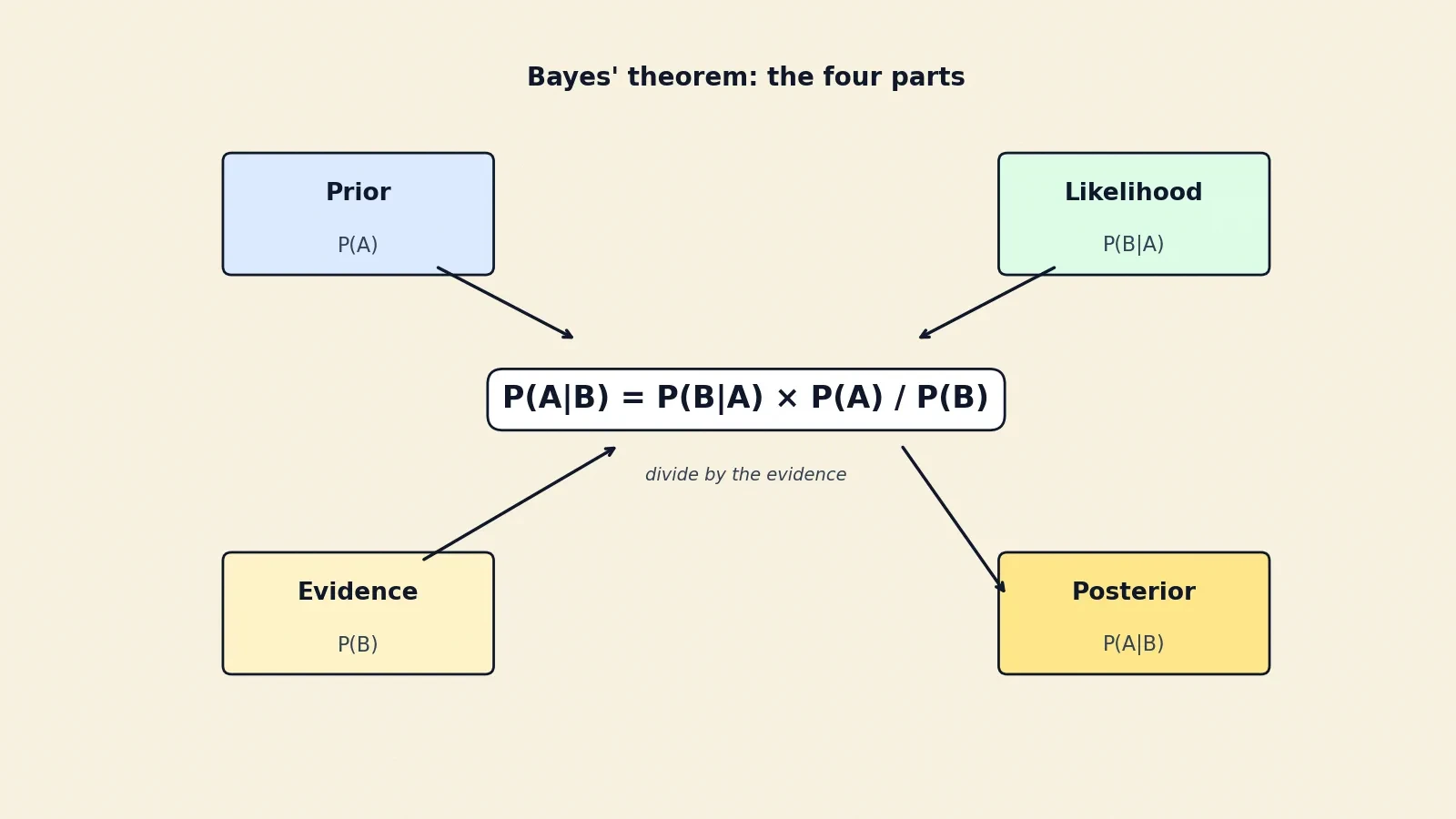
The formula is P(A|B) = P(B|A) x P(A) / P(B). Read the vertical bar as the words "given that". P(A|B) is the probability of A given that B has happened. P(B|A) is the probability of B given that A has happened. The formula says: the probability of A given B equals the probability of B given A, times the probability of A, divided by the probability of B.
Each piece has a name, and the names matter, because they are the vocabulary the rest of the article uses. P(A|B) is the posterior, the probability of A after seeing the evidence B. P(B|A) is the likelihood, the probability of seeing the evidence if A is true. P(A) is the prior, the probability of A before the evidence arrived. P(B) is the evidence, sometimes called the marginal likelihood, the total probability of seeing B under every possibility, and it acts as a normalising constant that makes the answer come out as a proper probability. The OpenStax introduction to probability theory states the same formula and the same four names, and it is a good place to check them against a second source.
The derivation takes two lines, and it is worth seeing, because it shows that Bayes' theorem is not a trick. It is a rearrangement of the definition of conditional probability — the same algebra you use to solve for an unknown, which our Algebra article works through from first principles. The probability of A given B is the probability of A and B together, divided by the probability of B. And the probability of A and B together is the probability of B given A, times the probability of A. Put those two facts together and the formula falls out. Nothing has been assumed, nothing has been smuggled in. The theorem is a consequence of the definition, the way a shadow is a consequence of the object that casts it.
Here is the formula in words, as a sentence you can carry around. The chance that a hypothesis is true, after seeing the evidence, equals how well the hypothesis predicts the evidence, times how likely the hypothesis was in the first place, divided by how likely the evidence was overall. If the hypothesis predicts the evidence far better than its rivals do, the posterior goes up. If the hypothesis was unlikely to begin with, the posterior stays low even after good evidence. The formula weighs the new against the old, and neither is allowed to shout down the other.
Most people get the direction of the formula backwards at first, and that confusion is the single most important misunderstanding in this article. P(B|A) is not P(A|B). The probability of a positive test given disease is not the probability of disease given a positive test. The first is a property of the test. The second is the number the patient actually wants. Confusing the two is like confusing the chance that a fire alarm sounds when there is a fire with the chance that there is a fire when the alarm sounds. The alarm almost always sounds during a fire, and it also sounds during burnt toast. The two numbers live in different worlds, and Bayes' theorem is the bridge between them.
Posterior is proportional to likelihood times prior
There is a shorter form of the rule that working statisticians use every day: the posterior is proportional to the likelihood times the prior. The denominator, P(B), is the same for every hypothesis you are comparing, because it is the total probability of the evidence. When you only want to know which hypothesis is more likely, you can drop it. The ranking of hypotheses is decided by likelihood times prior alone.
When you want an actual probability — a number like 9.02 percent, not just a ranking — the denominator comes back. It rescales everything so the probabilities add up to one. That is why the full formula has a division in it, and why the short form does not. Drop the denominator to compare, keep it to measure. Both forms are the same rule, used for different jobs.
This short form is also the reason Bayes' theorem feels so natural once you have used it a few times. It says: start with what you believed, multiply by how well each belief explains what you just saw, and then tidy up so the numbers add to one. That is how a sensible person updates, and it is how a careful scientist updates, and the formula is the precise version of the instinct. The instinct and the mathematics agree, which is rarer than it should be.
A first tiny example, before the big one
A toy example makes the machinery visible before the medical test puts it to work. Imagine two bags. The first bag holds nine white balls and one black ball. The second bag holds one white ball and nine black balls. You pick a bag at random — each bag equally likely — reach in without looking, and draw a white ball. Which bag did you probably pick?
Your first instinct says the first bag, and your instinct is right, but Bayes' theorem says how right. The prior for each bag is one half. The likelihood of drawing white from the first bag is nine in ten; from the second bag, one in ten. The posterior for the first bag is nine tenths times one half, divided by the total probability of drawing white, which is five tenths. That gives nine tenths, or 90 percent. A white ball makes the first bag nine times as likely as it was relative to the second, and the arithmetic says exactly how much the evidence moved you: from 50 percent to 90 percent.
The toy is small, but it carries the whole pattern. A prior, a likelihood, a posterior, and a denominator that collects every way the evidence could have happened. Keep that pattern in mind. The medical test in the next section is the same toy, with bigger numbers and higher stakes. The cab problem later in the article is the same toy again, with a witness instead of a bag. The spam filter near the end is the same toy once more, with words instead of balls. Learn the pattern once, and you will recognise it everywhere.
3. The Medical Test, Worked Step by Step
Now the centrepiece. Take a screening test for a disease that affects one person in a thousand. The test is 99 percent sensitive and 99 percent specific — about as accurate as screening tests get. A person tests positive. What is the chance they have the disease? Work it out by counting people, not by juggling percentages, and the answer stops being mysterious.
The four words you must not confuse
Four terms describe any diagnostic test, and confusing them is the root of the whole puzzle. Sensitivity is the proportion of people with the disease who test positive: true positives divided by all diseased people, true positives plus false negatives. Specificity is the proportion of people without the disease who test negative: true negatives divided by all healthy people, true negatives plus false positives. Positive predictive value is the proportion of people who test positive who really have the disease: true positives divided by all positive results, true positives plus false positives. Negative predictive value is the proportion of people who test negative who really are healthy: true negatives divided by all negative results. The positive predictive value is the posterior, the number the patient wants, and it is the only one of the four that depends on how common the disease is.
The StatPearls guide to diagnostic testing accuracy gives these four definitions in the standard form used in medical teaching, and it is worth reading if you want the clinical wording. The key fact to carry away is the split: sensitivity and specificity are properties of the test, and they do not change when the disease becomes rarer or commoner. Predictive values do change. A test can keep exactly the same sensitivity and specificity while its positive predictive value swings from 9 percent to 50 percent, depending only on who is being tested. That is not a flaw in the test. It is the arithmetic of rare events, and it is the whole point of this section.
The two-by-two table below lays out the four cells for the worked example. Read it as a grid: rows are what the test says, columns are what is actually true. The diagonal from top-left to bottom-right is where the test gets it right. The other diagonal is where it gets it wrong. Every number in the worked examples below comes from this table.
| Disease present | Disease absent | Total | |
|---|---|---|---|
| Test positive | 99 true positives | 999 false positives | 1,098 |
| Test negative | 1 false negative | 98,901 true negatives | 98,902 |
| Total | 100 | 99,900 | 100,000 |
Worked example 1: prevalence 1 in 1,000
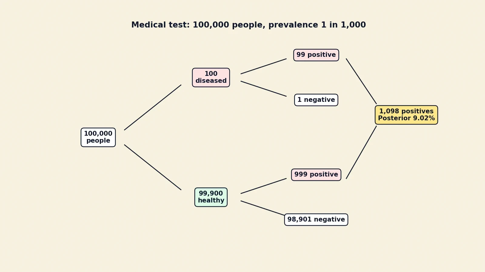
Take 100,000 people, chosen at random from a population where the disease affects one person in a thousand. Out of those 100,000 people, 100 have the disease and 99,900 do not. That is the prior, written as people instead of as a probability: one in a thousand, before any test is taken.
Now test everyone. Of the 100 people with the disease, the test catches 99 percent, so 99 test positive and 1 tests negative. Those 99 are the true positives. The 1 is a false negative, a sick person the test missed. Of the 99,900 healthy people, the test clears 99 percent, so 98,901 test negative and 1 percent — 999 people — test positive. Those 999 are the false positives, healthy people the test wrongly flagged.
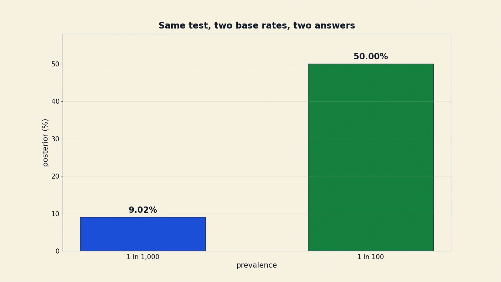
Add up the positives: 99 true positives plus 999 false positives gives 1,098 positive results in total. Of those 1,098 people, only 99 actually have the disease. The posterior, the chance of disease given a positive result, is 99 divided by 1,098, which is 9.02 percent. About 9 in 100 positive results are true. About 91 in 100 are false alarms.
Read that again, slowly, because it is the most important sentence in this article. A test that is right 99 percent of the time, in both directions, produces a positive result that is wrong 91 percent of the time. The reason is visible in the counting. The healthy group is 999 times larger than the sick group. Even a tiny error rate inside that huge group — one percent of 99,900 people — produces 999 false positives, which swamps the 99 true positives from the tiny sick group. The test is excellent. The disease is rare. Rarity wins.
The formula gives the same answer, as it must. Sensitivity times prevalence, divided by sensitivity times prevalence plus the false-positive rate times one minus prevalence, is 0.99 times 0.001, divided by 0.99 times 0.001 plus 0.01 times 0.999, which is 0.090164, or 9.02 percent. The frequency tree and the formula agree to every decimal place. Use whichever you find clearer; they are the same calculation in two costumes.
I have taught this example to students who were training for medical school, and I have watched the same thing happen every time. They do the counting themselves, on paper, in groups, and the room fills with a particular kind of protest. Someone always says the numbers must be wrong, because a 99 percent test cannot be wrong 91 percent of the time. Then someone else checks the multiplication, finds it correct, and the protest turns into a long silence. That silence is the sound of a base rate arriving in a person's thinking for the first time. It is worth more than any definition I could give them, because they found it themselves, in the arithmetic.
Worked example 2: the same test at prevalence 1 in 100
Now change one thing, and nothing else. Take the same test, with the same 99 percent sensitivity and 99 percent specificity, and use it in a population where the disease affects one person in a hundred instead of one in a thousand. Same test, same positive result. Different answer.
Out of 100,000 people, 1,000 now have the disease and 99,000 do not. Of the 1,000 sick people, 99 percent test positive, giving 990 true positives and 10 false negatives. Of the 99,000 healthy people, 1 percent test positive, giving 990 false positives and 98,010 true negatives. Total positives: 990 plus 990, which is 1,980. The posterior is 990 divided by 1,980, which is exactly 50 percent.
The same test, the same positive result — 9 percent in one population, 50 percent in another. Only the base rate changed. Nothing about the test moved. Nothing about the person moved. The prior moved, and the posterior followed it. This is the cleanest demonstration in the whole article that a test result has no meaning without a prior. A positive result is not a number. It is a number plus a population.
The comparison also shows why screening the general population and testing people with symptoms are different activities, even when the test is identical. A person who walks into a clinic with symptoms already has a higher prior than a person picked at random off the street, and the same positive result means more for them. Doctors know this instinctively, which is why they ask about symptoms and history before they order a test. They are estimating the prior. Bayes' theorem is the formal version of that clinical habit.
Why this is not a flaw in the test
It is tempting to conclude that the test is useless, or that screening is a waste of time. That conclusion is wrong, and it is worth saying so plainly. The test did real work. Before the test, the chance of disease was 0.1 percent. After a positive result, it is 9.02 percent. The test multiplied the chance by about ninety. A ninety-fold rise in probability is a powerful piece of evidence. It is simply not the same thing as a diagnosis, and nobody should treat it as one.
A positive result from a screening test is the start of an investigation, not the end of one. The normal next step is follow-up testing: a more specific confirmatory test, a clinical examination, a second sample. Screening tests are designed to be sensitive, to catch almost everyone with the disease, and that sensitivity is bought with false positives. Confirmatory tests are designed to be specific, to rule those false positives out. The two kinds of test do different jobs, and a screening programme that uses only one of them is doing half the work.
That is the false positive paradox, in its proper form. Even a very accurate test produces mostly false positives when the condition is rare. The paradox dissolves the moment you count people instead of staring at percentages. Count the sick, count the healthy, count the errors in each group, and the answer falls out. The percentages hide the base rate. The people reveal it.
4. The Minister Who Never Published: Thomas Bayes and Richard Price
The rule you have just used was written down by a man who never published it, in a paper his friend found among his belongings after his death. That is not a romantic exaggeration. It is the documented history, and it explains why the theorem carries the name of a person who never claimed it, in a form he never wrote.
Bayes the man
Thomas Bayes was born around 1701 — no birth date is known, and no birthplace can be stated with confidence, so this article gives neither — the eldest son of the Reverend Joshua Bayes and Ann Carpenter, a prominent Nonconformist family from Sheffield. He enrolled at the University of Edinburgh in 1719 to study logic and theology, because Nonconformists were barred from Oxford and Cambridge. From about 1733 or 1734 until he retired in 1752, he was minister of the Presbyterian Mount Sion Chapel at Tunbridge Wells in Kent, and he continued to live in Tunbridge Wells until his death.
Bayes was elected a Fellow of the Royal Society in 1742, for a 1736 work defending Newton against Bishop Berkeley, An Introduction to the Doctrine of Fluxions. He published only two works in his lifetime: a theological work, Divine Benevolence, in 1731, and the anonymous 1736 defence of fluxions. He died on 7 April 1761, aged 59, in Tunbridge Wells, and was buried in Bunhill Fields burial ground in London. A note on that date: some older sources print 17 April, which is a clerical error that has been copied from one reference work to another. The tombstone says 7 April, and 7 April is the date this article uses.
There is something quietly remarkable about this life. Bayes was a provincial minister who did mathematics in his spare time, published almost nothing, and died without knowing that his most important idea would survive him. He was not a professor chasing priority. He was a thoughtful man working on a hard problem — how to reason backwards from observed events to their unknown causes — because the problem interested him. The history of science has a handful of such figures, people whose best work reached the world only because someone else cared enough to carry it there. Bayes is one of them, and the someone else was Richard Price.
The essay found in his papers
After Bayes died, his friend Richard Price found an essay among his papers, edited it, wrote an introduction, and sent it to the Royal Society in a letter to John Canton, the Society's secretary. The essay was read to the Royal Society on 23 December 1763 and published in 1764, in volume 53 of the Philosophical Transactions, on pages 370 to 418. The volume is the volume for the year 1763, which is where the confusion comes from. People see the volume year and say the essay was published in 1763. It was read in 1763 and published in 1764, and the distinction is worth getting right, because it is one of those small errors that gets copied endlessly once it enters circulation.
The full title as printed in the journal was "An Essay towards solving a Problem in the Doctrine of Chances". It is a modest title for an ambitious paper. Bayes stated his own problem plainly: given the number of times an unknown event has happened and failed, find the chance that the probability of its happening in a single trial lies between any two named degrees of probability. In modern language, he was asking how to put a probability distribution on an unknown probability, after watching a run of successes and failures. That question — how to learn about a hidden chance from what you can see — is the heart of the whole subject.
Price did more than forward the manuscript. He added an introduction, footnotes, an abridgement of the latter part, and an appendix of numerical examples. The published Essay runs to 49 pages: 24 by Bayes and 25 by Price. Half the paper that carries Bayes' name was written by his friend. Price also applied the reasoning himself, using it in his 1767 Four Dissertations to answer the philosopher David Hume on the subject of miracles. That application is a matter of record, though the theological argument it was aimed at is beyond the scope of this article, and Bayes' theorem settles no question of theology. It is a rule for weighing evidence. What the evidence is about is a separate matter.
The offprint title
Here is a detail that changes how the paper should be understood. The offprint of the Essay — the separate copies printed for circulation — carried a different and more ambitious title: "A Method of Calculating the Exact Probability of All Conclusions founded on Induction". The historian Stephen Stigler established this in 2013, from surviving offprints, in a paper in Statistical Science whose DOI is 10.1214/13-STS438. Price's follow-up paper of 1765 carried a matching offprint title, "A Supplement to the Essay on a Method of Calculating the Exact Probability of All Conclusions founded on Induction".
That title matters, because it shows what Bayes and Price thought they were doing. They were not presenting a clever formula for updating odds. They were proposing a method for induction itself — for drawing general conclusions from particular observations, with a number attached to how confident you should be. The problem of induction had haunted philosophy since Hume, and here was a mathematical answer, or at least the beginning of one. The formula that now carries Bayes' name is a small part of that larger project, and the paper's real ambition was far bigger than the equation most textbooks print.
The billiard-table thought experiment
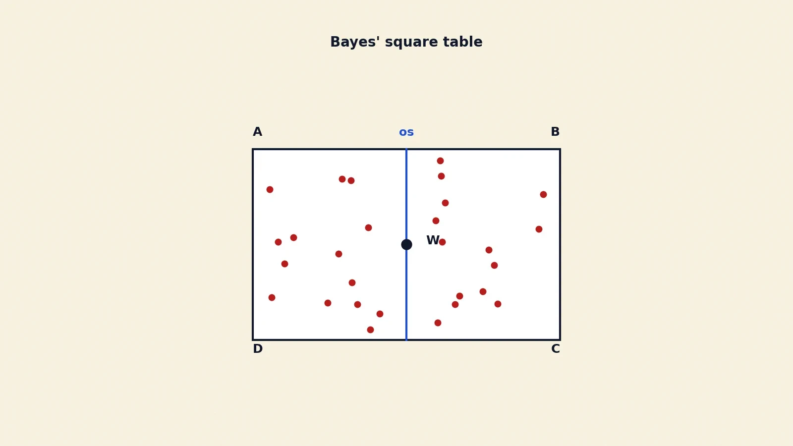
Bayes explained his idea with a thought experiment, and the thought experiment has been retold so often that the retelling has replaced the original. Here is the original, as Bayes wrote it. Imagine a square table, labelled ABCD, levelled so that a ball thrown onto it is equally likely to come to rest on any equal part of its surface. A ball, called W, is thrown first. Through the point where it rests, a line is drawn parallel to one side of the square. Then a second ball, called O, is thrown repeatedly. Each time O comes to rest on one side of the line is counted as the happening of an event. From the counts of happenings and failures, Bayes asked what could be said about where the line lies — that is, about the unknown probability.
Two things need saying about this picture. First, Bayes never mentions billiards anywhere in the Essay. The "billiard table" label is a later popularisation, and it is a misleading one, because a billiard table has pockets and cushions and a shape of its own, while Bayes' table is a featureless square chosen precisely because every part of it is the same as every other part. This article calls it the billiard-table thought experiment only because readers will recognise the name, and it says plainly here that Bayes himself described a square table, not a billiard table.
Second, Bayes assumed that the unknown probability was equally likely to take any value between zero and one — a uniform prior, in modern language — and he gave an argument for that assumption that is often overlooked. In modern integral notation, his result is that the probability the unknown chance lies between two values, after a given number of successes and failures, is the ratio of two integrals: the integral over that range of the unknown chance raised to the power of the successes, times one minus the chance raised to the power of the failures, divided by the same integral over the whole range from zero to one. Bayes did not use that notation. He worked with areas under curves, in the geometric style of his time. The integrals are a translation, not a quotation.
The modern retelling, in the form popularised by the statistician David Spiegelhalter in The Art of Statistics, runs like this: a white ball is thrown at random onto a table, its position is marked with a line, and the white ball is removed. Red balls are then thrown, and you are told only how many land to the left of the line and how many to the right. Where is the line, and what is the probability that the next red ball falls to the left of it? That version is easier to picture, and it is a faithful retelling of the same mathematics, but it is a retelling. The original is the square table, the ball W, the line, and the ball O, thrown again and again.
Laplace, the second discoverer
The story does not end with Bayes, because the idea was discovered twice. Pierre-Simon Laplace, working in France, independently reached the same result and published it in 1774, in a memoir on the probability of causes given events. He was apparently unaware of Bayes' work at that point. Laplace stated the principle in words, not with the modern equation: the probability of a cause given an event is proportional to the probability of the event given its cause. He refined the result in further memoirs, and summarised it in his great Theorie analytique des probabilites in 1812, with a popular exposition, the Essai philosophique sur les probabilites, in 1814, based on a lecture from 1794.
Laplace also did something Bayes never did: he used the method on real data, at scale. He applied it to birth records — the fact that more boys than girls are born — across Paris, London, Naples, St Petersburg, and rural France, and concluded by 1812 that a higher boy birth rate was a general law. That was the first large-scale demonstration that inverse probability could answer a question about the real world, not just about balls on a table.
And here is the correction that this section owes the reader. Bayes never wrote the modern formula. His Essay states a special case — what modern retellings call Proposition 9 — about limits on an unknown probability after a given number of successes and failures. Laplace gave the general modern form. The name "Bayes' theorem" is anachronistic: the paper contains a special case of a general conditional-probability result, and the modern name and form came later, largely through Laplace and the writers of the nineteenth and twentieth centuries. The Bayesian interpretation of probability was developed mainly by Laplace, and about two centuries later Harold Jeffreys put Bayes' algorithm and Laplace's formulation on an axiomatic basis.
None of that diminishes Bayes. He asked the question first, and he answered it in the case that mattered most to him. Laplace generalised the answer and showed the world how to use it. Between them, they gave science a way to reason backwards from what it can see to what it cannot, and that way of reasoning sat mostly unused for a century and a half, waiting for computers to make it practical. The best popular history of that long wait is Sharon Bertsch McGrayne's The Theory That Would Not Die, published by Yale University Press in 2011, which traces the idea from its discovery in the 1740s through Laplace, through a hundred and fifty years of near-taboo, through wartime use, and into the computer revival of the 1980s.
5. Prior, Likelihood, Evidence, Posterior: The Four Characters
Every application of Bayes' theorem is a small drama with four characters. Learn them by name, and every worked example in this article becomes a matter of casting the right number in the right role.
The prior
The prior is the probability of a hypothesis before the evidence arrives. In the medical test, the prior is one in a thousand — the prevalence of the disease in the population being tested. It is the answer to the question: before I knew anything about this person, how likely was this?
The prior is the character people forget, and forgetting it is the whole fallacy this article is about. A positive test feels like strong evidence, and it is, but strong evidence multiplied by a tiny prior still gives a small posterior. A test that multiplies your belief by ninety still leaves you at 9 percent if you started at 0.1 percent. The prior sets the scale. Everything else moves within it.
The likelihood
The likelihood is the probability of seeing the evidence if the hypothesis is true. In the medical test, the likelihood of a positive result given disease is 99 percent — the sensitivity. It answers the question: if the disease were present, how often would I see exactly this result?
The likelihood is where the test itself lives. A good test has a high likelihood for the right hypothesis and a low likelihood for the wrong ones. Sensitivity is the likelihood of a positive result when the disease is present. One minus specificity — the false-positive rate — is the likelihood of a positive result when the disease is absent. The gap between those two numbers is the test's power. When the gap is wide, the evidence moves you far. When the gap is narrow, it barely moves you at all.
The evidence
The evidence, P(B), is the total probability of seeing the result under every hypothesis at once. In the medical test, it is the 1,098 positives in 100,000 people — the true positives plus the false positives, all the ways a positive result can happen. It answers the question: how often would I see this result anyway, regardless of which hypothesis is true?
The evidence is the least glamorous of the four characters, and it does the quiet work of keeping the answer honest. It is the denominator that turns a comparison into a probability. Without it, you can say which hypothesis is more likely. With it, you can say how likely, in numbers that add up to one. When people skip the denominator, they usually do so because it is the hardest piece to compute — it requires thinking about every alternative, not just the favourite one — and that skipping is where most errors creep in.
The posterior
The posterior is the probability of the hypothesis after the evidence has been seen. In the medical test, it is 9.02 percent — the chance of disease given a positive result. It is the answer the patient wants, the number the whole calculation exists to produce. It answers the question: now that I have seen this, how likely is this?
The posterior has one more property, and it is the most important property in the article. Today's posterior is tomorrow's prior. When a second piece of evidence arrives, you do not start over. You start from where the first piece left you, and you update again. That is the subject of Section 7, and it is what turns Bayes' theorem from a single calculation into a way of learning.
The prior is not a guess
One more point, before the odds form arrives. The prior is not a guess, and the charge that Bayes' theorem is unscientific because it uses one is a misunderstanding worth answering directly. A prior must be justified. It can come from a measured base rate, like the prevalence of a disease or the proportion of cabs of each colour in a city. It can come from a symmetry argument, like Bayes' own uniform prior on the square table, where every position is as likely as every other. Or it can come from an explicitly stated assumption that the reader can inspect, challenge, and replace with their own. An unjustified prior is a flaw in the analysis, not a flaw in the theorem. A prior that is written down, sourced, and open to argument is the opposite of a guess. It is the most honest part of the calculation, because it is the part where the analyst says, in public, what they believed before the evidence arrived.
6. The Odds Form: How to Update in Your Head
There is a second form of Bayes' theorem, and it is the one to use when you want to update a belief in your head, without a calculator. It works in odds instead of probabilities, and it turns the whole calculation into a single multiplication.
Posterior odds equal prior odds times the likelihood ratio
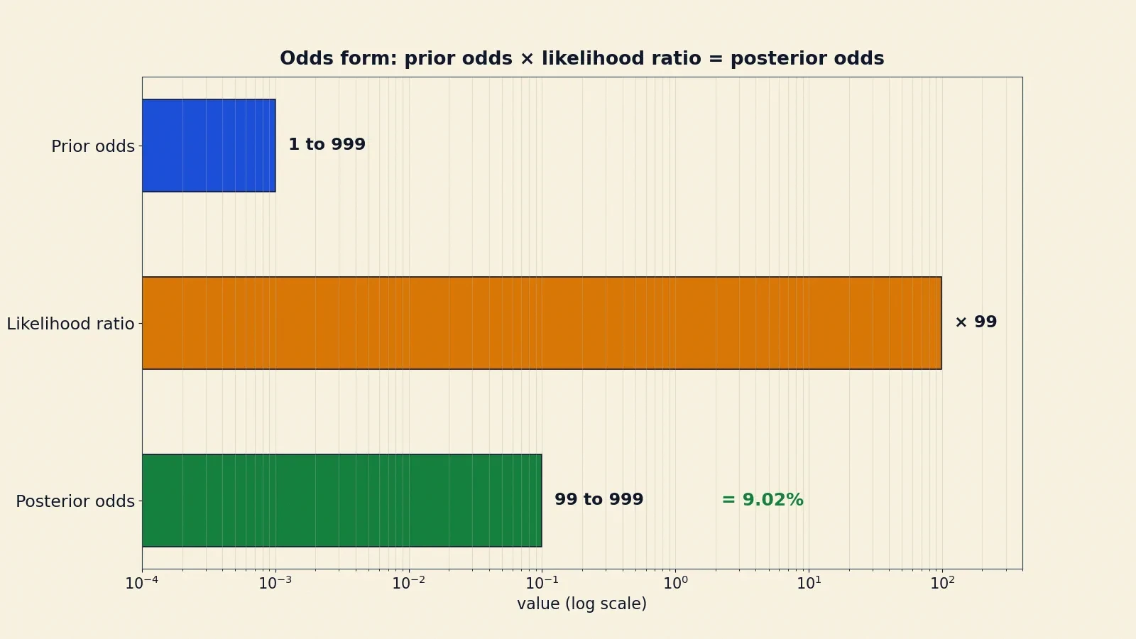
The odds form says: posterior odds equal prior odds times the likelihood ratio. In symbols, the odds of a hypothesis given the evidence equal the odds of the hypothesis before the evidence, multiplied by the probability of the evidence if the hypothesis is true, divided by the probability of the evidence if the hypothesis is false. The ratio at the end is called the likelihood ratio, and in the two-hypothesis form it is also called the Bayes factor.
Take the medical test again. The prior odds of disease are 1 to 999 — one sick person for every 999 healthy ones. The likelihood ratio for a positive result is the sensitivity divided by the false-positive rate: 0.99 divided by 0.01, which is 99. Multiply them: 1 to 999, times 99, gives posterior odds of 99 to 999. Convert odds back to a probability by dividing the first number by the sum of the two: 99 divided by 99 plus 999, which is 99 divided by 1,098, which is 9.02 percent. The same answer, reached by one multiplication and one division.
The odds form is worth learning because it separates the two jobs cleanly. The prior odds say what you believed. The likelihood ratio says what the evidence is worth. Multiply them, and you have what you should believe now. When a second piece of evidence arrives, multiply again. The odds form is the arithmetic of changing your mind, and it is short enough to do on the back of an envelope.
The Bayes factor
The likelihood ratio, or Bayes factor, is a number with a plain reading. Greater than one, the evidence favours the hypothesis. Equal to one, the evidence changes nothing. Less than one, the evidence counts against the hypothesis. A Bayes factor of 99, like the medical test's, is strong evidence. A Bayes factor of 2 is weak evidence. A Bayes factor of 0.5 is evidence against, halving the odds.
Take the mammography example, which Section 10 works through in full. The prior odds of breast cancer in the screening group are 1 to 99. The likelihood ratio of a positive mammogram is the sensitivity, 90 percent, divided by the false-positive rate, 9 percent, which is 10. Multiply: 1 to 99, times 10, gives posterior odds of 10 to 99. Convert to a probability: 10 divided by 109, which is about 9.2 percent. The test multiplied the odds by ten, and ten times a small number is still a small number. That is the whole story, in one multiplication.
The Bayes factor also has a practical virtue. It does not depend on the prior at all. Two people who disagree about the prior can agree about the Bayes factor, because it is a property of the evidence and the test, not of their beliefs. They can argue about where to start, and still agree about how far the evidence moves them. That separation — what you believed, against what the evidence is worth — is one of the most useful habits Bayes' theorem teaches.
Multiplying evidence
Each independent clue is another likelihood ratio, multiplied in. That is how the odds form scales from one test to many. A second test with a likelihood ratio of 5 multiplies the odds by 5 again. A third clue with a likelihood ratio of 0.2 divides them by 5. The posterior after all the evidence is the prior odds, multiplied by every likelihood ratio in turn.
This is the bridge to the two great applications later in the article. A spam filter multiplies the likelihood ratios of fifteen words to reach a verdict on an email. A search team multiplies the likelihood ratios of sonar contacts, drift models, and previous search effort to reach a probability map of the ocean floor. The arithmetic is the same in both cases. Only the evidence changes.
There is a neat companion idea worth one sentence, because it connects this article to its neighbour. Take the logarithm of the odds, and multiplication becomes addition: each piece of evidence adds its log likelihood ratio to the running total. Our Logarithms article explains why logarithms turn multiplication into addition, and that is exactly what happens here — updating a belief becomes a matter of adding up small scores, one per clue.
7. Updating Again and Again: Sequential Learning and Conjugate Priors
Bayes' theorem is not a one-off calculation. It is a loop. Each new piece of evidence updates the previous posterior, and the result becomes the prior for the next round. That loop is how learning actually happens, and it is where the theorem earns its keep.
Today posterior is tomorrow prior
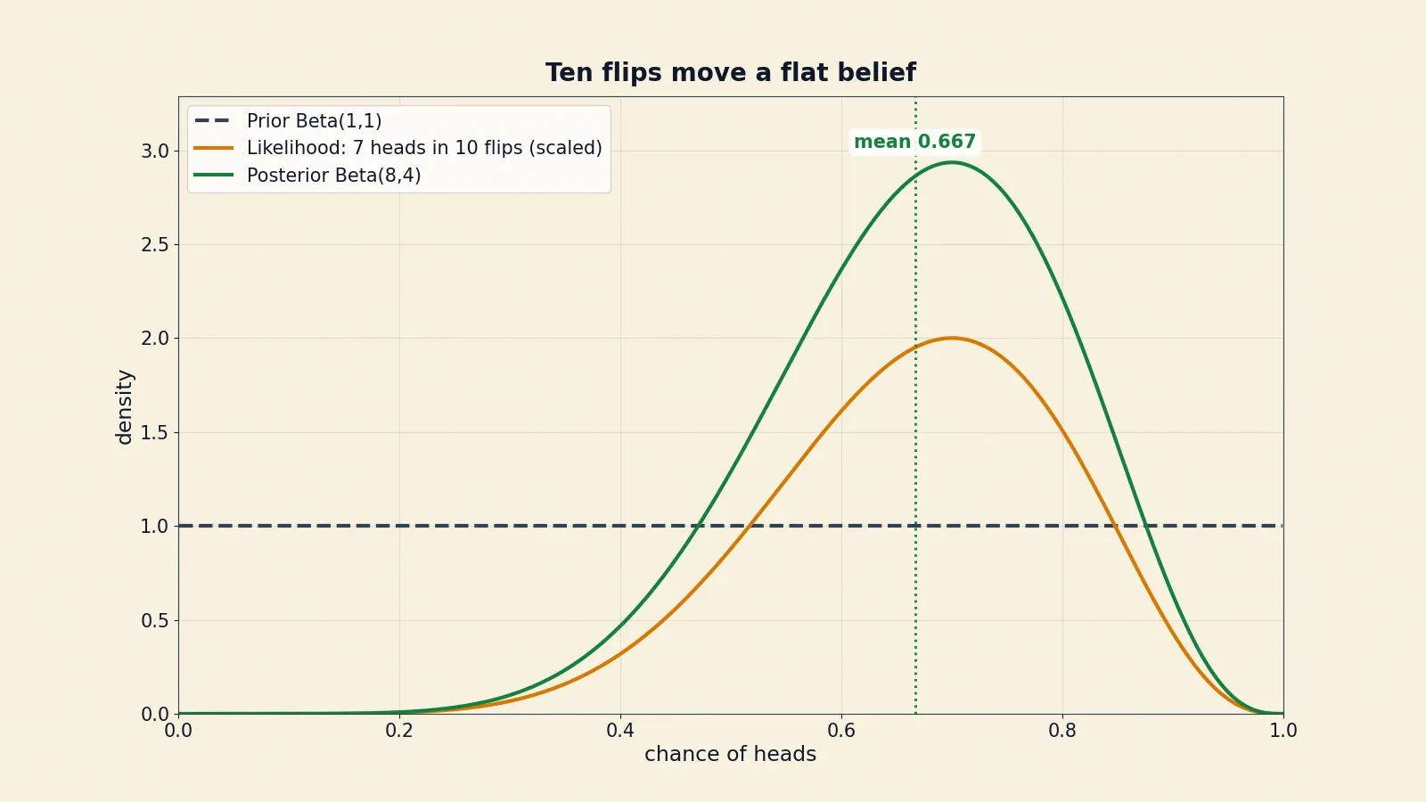
The cleanest way to see the loop is a coin. Suppose you have a coin, and you do not know whether it is fair. You start with a flat prior: every value of the coin's chance of landing heads, from zero to one, is equally likely. In the language of the next subsection, that is a Beta(1,1) prior, with a mean of 0.5.
Flip the coin once, and it lands heads. The posterior is now a Beta(2,1) distribution, with a mean of 0.667. One head has moved your best guess from 0.5 to about two thirds. Flip it again, and it lands heads again. The posterior is now Beta(3,1), with a mean of 0.75. Two heads in a row, and your best guess has climbed to three quarters.
Keep going. Ten flips, seven heads and three tails, and the posterior is Beta(8,4), with a mean of 8 divided by 12, which is 0.667. Notice what happened. The first head pulled the mean sharply upward, because there was almost no data and the prior was flat. The later flips pulled it back down toward the observed proportion, seven in ten. With little data, the prior weighs heavily. With more data, the data dominate. That is the loop doing its work, one flip at a time.
I keep a coin on my desk, and I have run this experiment with students more times than I can count. The first flip always produces the biggest argument. Someone says the coin must be biased. Someone else says one flip proves nothing. Both are half right, and Bayes' theorem is the referee: one flip moves you, but not far, and the size of the move is exactly the size the arithmetic says. By the tenth flip, the argument is over. The numbers have spoken, and everyone in the room can see how far they have moved, and why.
The order of the evidence does not matter for the final posterior, given the same total evidence and the same model. Seven heads and three tails give Beta(8,4) whether the heads came first or last. That is reassuring, and it is also a check on the method: a rule for learning should not depend on the order in which you happened to learn things.
Conjugate priors in plain language
Updating would be tedious if every new piece of evidence required a fresh integral. For certain pairings of prior and likelihood, it does not. These are called conjugate priors, and for them the posterior belongs to the same family as the prior, so updating becomes simple arithmetic.
The beta distribution is conjugate to the binomial likelihood. A Beta(a, b) prior, plus s successes and f failures, gives a Beta(a plus s, b plus f) posterior. The numbers a and b act as prior pseudo-counts, phantom earlier observations. Beta(1,1) is a uniform prior — one phantom head and one phantom tail, which is the same as knowing nothing. Beta(2,2) behaves like two phantom heads and two phantom tails. Updating is just adding counts: add the heads you saw to a, add the tails to b, and you are done. The coin example above is exactly this rule, worked three times.
The table below lists the pairings worth knowing. Keep it to three rows. The first is the one this article uses. The other two are there so you know the pattern is general, not a trick of the coin.
| Likelihood | Prior | Posterior |
|---|---|---|
| Binomial (counting successes) | Beta | Beta, with counts added |
| Poisson (counting events) | Gamma | Gamma, with counts added |
| Normal (measuring a mean, known variance) | Normal | Normal, with precision added |
Why this matters
Conjugate priors matter for two reasons. The practical reason is that they make updating cheap: add the counts, and the posterior is ready. Before fast computers, that cheapness was the difference between a method you could use and a method you could only admire. The conceptual reason is deeper. The pseudo-counts make the prior honest. A Beta(1,1) prior says, in effect, "I have seen one head and one tail before we started." A Beta(100,100) prior says, "I have seen a hundred of each." The second prior is far harder for new data to move, and the arithmetic shows exactly how much harder. A prior is not a vague feeling. It is a weight, measured in phantom observations, and the reader can see the weight and judge whether it is fair.
That weight fades as data accumulate. With ten flips, a Beta(1,1) prior still matters. With a thousand flips, it is invisible. With a lot of data, Bayesian and frequentist answers converge, provided the prior does not rule out plausible values. That convergence is the bridge to Section 13, where the two schools of statistics are compared properly. For now, hold on to the picture: the prior is a starting position, the data are a pull, and the posterior is where you end up when the pulling stops.
Bayes' own result on the square table was, in effect, a conjugate update, though he did not have the word for it. His uniform prior on the unknown chance, updated by the counts of the ball O landing on each side of the line, is the Beta(1,1) case in geometric dress. The integrals he computed with areas under curves are the same integrals a modern student computes by adding counts — and the area-under-a-curve idea is the heart of integration, which our Calculus article explains in full. The notation changed. The idea did not.
8. The Base Rate Fallacy: Why Smart People Get This Wrong
If Bayes' theorem is so simple, why do so many people get its answers wrong? The reason has a name: the base rate fallacy, also called base rate neglect. It is the tendency to ignore general statistical information about how often something occurs in a population — the base rate, the prior — in favour of vivid, case-specific information. A witness who sounds confident, a test result printed in bold, a description that fits a stereotype: these are vivid, and they push the base rate out of mind.
The psychologists Daniel Kahneman and Amos Tversky demonstrated the fallacy in a series of experiments in the 1970s, and they traced it largely to the representativeness heuristic — judging by similarity to a stereotype instead of by statistical likelihood. Something that looks like a librarian feels like a librarian, even when librarians are rare and the population is full of farmers. Something that looks like a disease feels like a disease, even when the disease is rare and the population is full of healthy people. The resemblance is real information, but it is not the only information, and it is not the information that matters most. The correct method is Bayes' theorem: weigh the prior against the new evidence, and let the arithmetic decide how far to move.
We cover the base rate fallacy briefly in our Misleading Statistics article; here is the full story, with the two classic experiments. The definition fits in one paragraph, and it is the paragraph above. Everything after this section is the evidence for it: a witness, a mammogram, and a courtroom. Do not re-explain the fallacy at length after this point. The examples do the explaining.
One laboratory example shows the mechanism in its purest form. In a famous experiment, Kahneman and Tversky gave people a description of a man called Steve — "very shy and withdrawn, invariably helpful, but with little interest in people, or in the world of reality. A meek and tidy soul, he has a need for order and structure, and a passion for detail" — and asked what his occupation was, from a list including farmer, salesman, airline pilot, librarian and physician. People guessed he was a librarian, even though there are far more male farmers than male librarians in the population. The description was vivid. The base rate was dull. The vivid won. That is the fallacy in miniature, and it is the same error, in a different costume, as guessing 99 percent for the medical test and 80 percent for the cab.
9. The Cab Problem: An 80 Percent Reliable Witness Who Is Probably Wrong
A cab was involved in a hit-and-run accident at night. Two companies operate in the city: Green and Blue. A witness identified the cab as Blue. The witness was tested under the same night conditions, and correctly identified each colour 80 percent of the time. Question: what is the probability that the cab was Blue rather than Green?
Before you read on, guess. Most people answer 80 percent, the reliability of the witness. That answer is wrong, and the reason it is wrong is the same reason the medical test surprised you. The witness is the likelihood. The colours of the cabs are the prior. And the prior is doing most of the work.
The setup, with the correct numbers
Here are the numbers, and they matter enough to state with care. Eighty-five percent of the cabs in the city are green, and 15 percent are blue. The witness identified the cab as Blue, and the witness is right 80 percent of the time and wrong 20 percent of the time, for each colour. That is the whole setup. Nothing is hidden.
The classic statement of this problem comes from Tversky and Kahneman's 1982 paper on the evidential impact of base rates, and from Kahneman's retelling in Thinking, Fast and Slow, chapter 16. The numbers have been mangled in some retellings, with the colours reversed, and the reversal destroys the point of the example. With green cabs in the majority, the answer is about 41 percent. With the colours the other way round, the answer would be about 96 percent, and the puzzle would vanish. The draft of this article was checked against the original sources to make sure the colours are the right way round: 85 percent green, 15 percent blue.
The frequency tree
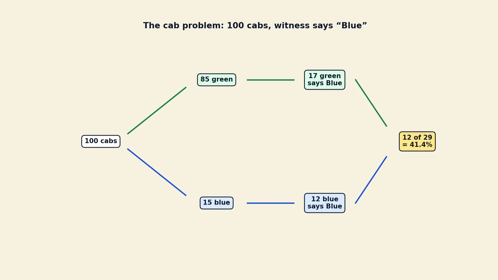
Count cabs, the way you counted people for the medical test. Out of 100 cabs, 85 are green and 15 are blue. The witness says "Blue" for 12 of the 15 truly blue cabs, because the witness is right 80 percent of the time, and 15 times 0.8 is 12. The witness also says "Blue" for 17 of the 85 green cabs, because the witness is wrong 20 percent of the time, and 85 times 0.2 is 17. Total "says Blue" is 29. Of those 29, only 12 are truly blue. The posterior is 12 divided by 29, which is 41.4 percent.
The cab was more likely green — 58.6 percent — despite the witness. An 80 percent reliable witness, testifying in the plainest terms, is probably wrong. The witness is not lying, and the witness is not incompetent. The witness is 80 percent reliable, and 80 percent reliability is not enough to overcome a base rate of 85 to 15. The green cabs are so numerous that their 20 percent error rate produces more false "Blue" reports than the blue cabs produce true ones. It is the medical test again, with headlights instead of blood samples: the huge group produces more errors than the tiny group produces correct answers.
I have asked this question at dinner tables, in classrooms, and in conference hallways, and I have never once had a first guess below 70 percent. People trust the witness. They picture a person standing on a street corner, pointing at a blue cab, and the picture feels like evidence. The base rate — a dull fact about the composition of a taxi fleet — feels like background noise. Bayes' theorem says the background noise is the main signal, and the confident witness is the garnish. That reversal is hard to feel, which is why the arithmetic has to be done out loud, with cabs counted on fingers, before anyone believes it.
The reversed-colours twist
Suppose the numbers were reversed, and blue cabs made up 85 percent of the fleet, with green cabs at 15 percent. The witness says "Blue", with the same 80 percent reliability. Now the frequency tree gives 68 truly blue cabs identified correctly, plus 3 green cabs misidentified, for 71 "says Blue" reports, of which 68 are truly blue. The posterior is about 96 percent. The same witness, the same reliability, the same words — and the answer swings from 41 percent to about 96 percent. The witness did not change. The base rate changed, and the base rate is doing the work.
That swing is the most useful fact in this section for anyone who has to judge evidence in real life. A witness, a test, a sensor, a tip-off: none of them has a reliability that means anything on its own. Reliability only becomes a probability when it meets a base rate. Ask for the base rate first, and the witness second, and you will be right far more often than the person who does it the other way round.
The causal version
Kahneman tells a second version of the same problem, and it is the most revealing part of the story. The numbers are identical, but the base rate is presented causally: the two companies run equal numbers of cabs, but Green cabs are involved in 85 percent of accidents. People use the base rate correctly in this version. They give answers close to 41 percent. The two versions are mathematically indistinguishable, and psychologically very different.
The difference is that a causal base rate feels like information about the case, while a statistical base rate feels like background. "Green cabs are involved in 85 percent of accidents" sounds like a fact about this accident. "Eighty-five percent of cabs are green" sounds like a fact about the city. The mind treats the first as evidence and the second as scenery, even though the arithmetic is identical. That is the representativeness heuristic at work, and it is why the fallacy is so stubborn: it is not a failure of arithmetic. It is a failure of attention. The mind attends to what looks like a cause, and ignores what looks like a context, and Bayes' theorem is the discipline of attending to both.
10. Mammograms and the Doctors Who Got It Wrong
The medical test in Section 3 was a hypothetical, with clean numbers chosen for teaching. The mammography story is the same arithmetic, in the real world, with real doctors getting it wrong. It is the most important section in this article for anyone who will ever sit in a clinic, or read a test result, or trust a professional's interpretation of one.
The Gigerenzer numbers
Here is the setup, in the version used by the psychologist Gerd Gigerenzer in training courses for gynaecologists. One percent of the women in the screening group have breast cancer. If a woman has cancer, the test is positive in 90 percent of cases. If she does not have cancer, the test is still positive in 9 percent of cases. Question: a woman tests positive. What is the chance she has cancer?
Count women, the way you counted people before. Out of 1,000 women, 10 have cancer and 990 do not. Of the 10 with cancer, 9 test positive. Of the 990 without cancer, 9 percent test positive, which is 89 women. Total positives: 98. Of those 98, 9 have cancer. The posterior is 9 divided by 98, which is 9.2 percent. Roughly one in ten positive results is a true positive. Roughly nine in ten are false alarms.
That is the same arithmetic as the medical test in Section 3, with different numbers and the same conclusion. A test that catches 90 percent of cancers still gives a positive result that is wrong about 91 percent of the time, because cancer is rare in the screened population and the healthy group is large. The numbers are not the point. The pattern is the point, and the pattern is the base rate, quietly deciding the answer while everyone watches the test.
The physicians
The reason this example matters is not the arithmetic. It is who got the arithmetic wrong. In a 1982 study by David Eddy, 95 out of 100 physicians estimated the probability at 70 to 80 percent when given a version of the mammography numbers — in Eddy's version the sensitivity was 80 percent and the false-positive rate 9.6 percent, giving a correct answer of 7.8 percent. They were asked a question about a test, and they answered with the sensitivity, 80 percent, trimmed down a little for caution. They confused the probability of a positive test given cancer with the probability of cancer given a positive test — the same confusion, in a white coat, as the audience in my lecture hall.
Gigerenzer and his colleagues then showed that the problem is not the doctors. It is the format. In a 1998 study by Hoffrage and Gigerenzer, physicians were given a different screening problem — the hemoccult test for hidden blood in the stool, where the prevalence of colon cancer was 0.3 percent, the sensitivity 50 percent and the false-positive rate 3 percent, giving a correct answer of about 5 percent, or 1 in 20 positive results. With percentages, only 1 out of 24 physicians found the Bayesian answer. With natural frequencies — "1 out of 20" instead of "5 percent" — 16 out of 24 found it. The doctors did not get smarter between the two versions. The numbers got clearer. The Frontiers in Psychology paper on natural frequencies reports these findings and the wider research behind them, including the Eddy study and the Hoffrage and Gigerenzer experiment, and its DOI is 10.3389/fpsyg.2015.01473.
That result should change how anyone presents a risk. Percentages hide the base rate, because a percentage is a ratio with its denominator stripped away. "Ninety percent" does not say ninety percent of what. Natural frequencies keep the denominator visible: 9 out of 98. The moment you can see the 98, you can see the 89 false positives inside it, and the answer stops being a mystery. The doctors in the study were not innumerate. They were given numbers in a format that hid the very thing they needed to see.
Natural frequencies: the fix
The fix, then, is embarrassingly simple. Say "9 out of 98" instead of "9.2 percent". Say "99 out of 1,098" instead of "9.02 percent". Say "12 out of 29" instead of "41.4 percent". Counting people is easier than dividing probabilities, because people are the thing the probabilities are about. Gigerenzer's work is a long argument for that single habit, and it is an argument this article endorses without reservation.
There is a broader lesson here for anyone who communicates risk: a patient, a reader, a voter, a jury. The format of a number is part of the number. Present a risk as a percentage and people will anchor on the vivid figure. Present it as a frequency and they will see the population it came from. The same information, honestly presented in two ways, produces different understanding, and the difference is not small. It is the difference between 1 out of 24 and 16 out of 24 getting the right answer.
The thesis, in one picture
Step back and look at Sections 3, 9, and 10 together. A 99 percent test gives 9 percent. An 80 percent witness gives 41 percent. A 90 percent mammogram gives 9.2 percent. In every case, the vivid number — the sensitivity, the reliability — is high, and the correct answer is low, and the gap between them is the base rate. That gap is the subject of this article. Close it, and the surprises vanish. Leave it open, and even experts will fall into it, in clinics and in courtrooms, with consequences that are not academic at all.
11. When a Number Sends an Innocent Person to Prison: Sally Clark and the Prosecutor Fallacy
The base rate fallacy is not a parlour puzzle. In a courtroom, it can put an innocent person in prison. The case of Sally Clark is the proof, and it is told here in a factual tone, because the facts are grave enough without embellishment.
The case in brief
Sally Clark was a British solicitor. In November 1999 she was convicted of murdering her two infant sons, Christopher, aged 11 weeks, and Harry, aged 8 weeks. The defence said the children had died of sudden infant death syndrome, known as SIDS. The prosecution said she had killed them. The case turned, in large part, on a number.
The 1-in-73-million figure
The prosecution called the paediatrician Sir Roy Meadow, who testified that the chance of two children from an affluent family suffering SIDS was 1 in 73 million. He reached that figure by taking his estimate of 1 in 8,500 for a single SIDS death in similar circumstances, and squaring it. Eight thousand five hundred squared is 72,250,000. Meadow's more precise figure of 1 in 8,543 squared gives 72,982,849, about 1 in 73 million — the number quoted at trial. The arithmetic of the squaring was correct. Everything else about the number was wrong.
Squaring is only valid if the two events are independent — if the chance of the second death is the same whether or not the first has happened. That assumption was never justified, and it is false. Two children in one family share genetics and environment, and a second SIDS death after a first is far more likely than a first death in a family with no history of one. Later analysis put the chance of a second SIDS death after a first at roughly 1 in 60 to 1 in 100, not 1 in 8,500, so the true figure for two deaths was roughly a hundred times larger than 1 in 73 million. The squaring treated two deaths in one family as if they were two deaths in two unrelated families, drawn at random from the population. They were not.
The two errors
Meadow's figure carried two errors, and they are the two errors this article has been circling since Section 2. The first is the independence error: the squaring assumed the deaths were independent, and they were not. Shared genes and a shared home make the second death much more likely after the first, and no evidence was offered to justify treating them as independent. The second error is the prosecutor's fallacy: confusing the probability of the evidence given innocence with the probability of innocence given the evidence.
Put the second error in the language of this article. Even if the 1 in 73 million figure had been right, it would have been P(two SIDS deaths | innocent family), the chance of seeing this evidence if the family were innocent. The jury needed P(innocence | two deaths), the chance the family was innocent given that two deaths had happened. Those are different numbers, related by Bayes' theorem, and the relation runs through the prior — the base rate of mothers who murder two children, against the base rate of families who suffer two SIDS deaths. The prosecution presented the first number as if it were the second. It is the medical test confusion, in a courtroom, with a woman's freedom at stake.
The correction
On 23 October 2001, the Royal Statistical Society issued a public statement expressing concern at the misuse of statistics in the courts. It said the 1 in 73 million figure had no statistical basis, and that squaring would only be valid if SIDS cases arose independently within families, an assumption that would have to be justified empirically. In January 2002, the Society wrote to the Lord Chancellor making the same point.
"...has no statistical basis." — Royal Statistical Society, on the 1 in 73 million figure in the Sally Clark case, 23 October 2001
Clark's first appeal was dismissed in October 2000. Her convictions were overturned at a second appeal in January 2003, with judgment given on 11 April 2003, after it emerged that the prosecution pathologist, Alan Williams, had failed to disclose microbiological reports suggesting her younger son had died of natural causes, a Staphylococcus aureus infection. She had spent more than three years in prison. After the appeal, the Attorney General ordered a review of similar cases, and Donna Anthony and Angela Cannings, both convicted of murdering more than one of their children, also had their convictions overturned. Sally Clark died on 16 March 2007 of alcohol poisoning.
The case is the strongest argument in this article for taking Bayes' theorem seriously outside the classroom. A number that looks precise can be precisely wrong, and the wrongness can hide in the assumptions, not in the arithmetic. Meadow's multiplication was correct. His independence assumption was not, and his conditional was the wrong way round, and nobody in the courtroom caught either error until the damage was done. The lesson is not that statistics has no place in court. It is that statistics in court needs the same discipline as statistics anywhere else: state the prior, justify the independence, and check which way round the conditional runs. A jury that is told "1 in 73 million" without being told what that number is the probability of has been misled, however honestly the number was computed.
12. Bayes at Work: Spam, Submarines and Lost Airliners
So far the theorem has been a classroom tool and a courtroom warning. Now it goes to work. The same rule that sorts a positive test from a false alarm also sorts your email, finds lost submarines, and locates a missing airliner on the ocean floor. The settings change. The arithmetic does not.
Spam filters
In August 2002, the programmer Paul Graham published an essay called "A Plan for Spam", proposing that email could be filtered with a Bayesian combination of the spam probabilities of individual words. His method was simple. Start with two collections of email: one of spam, one of ordinary mail, called ham. For each word, estimate its spam probability from how often it appears in each collection. Take the fifteen most interesting words in a new message — the ones whose probabilities are furthest from a half — and combine their probabilities with Bayes' rule. Treat the message as spam if the combined probability is above 0.9. On his own mail, Graham's filter missed fewer than 5 per 1,000 spams, with zero false positives.
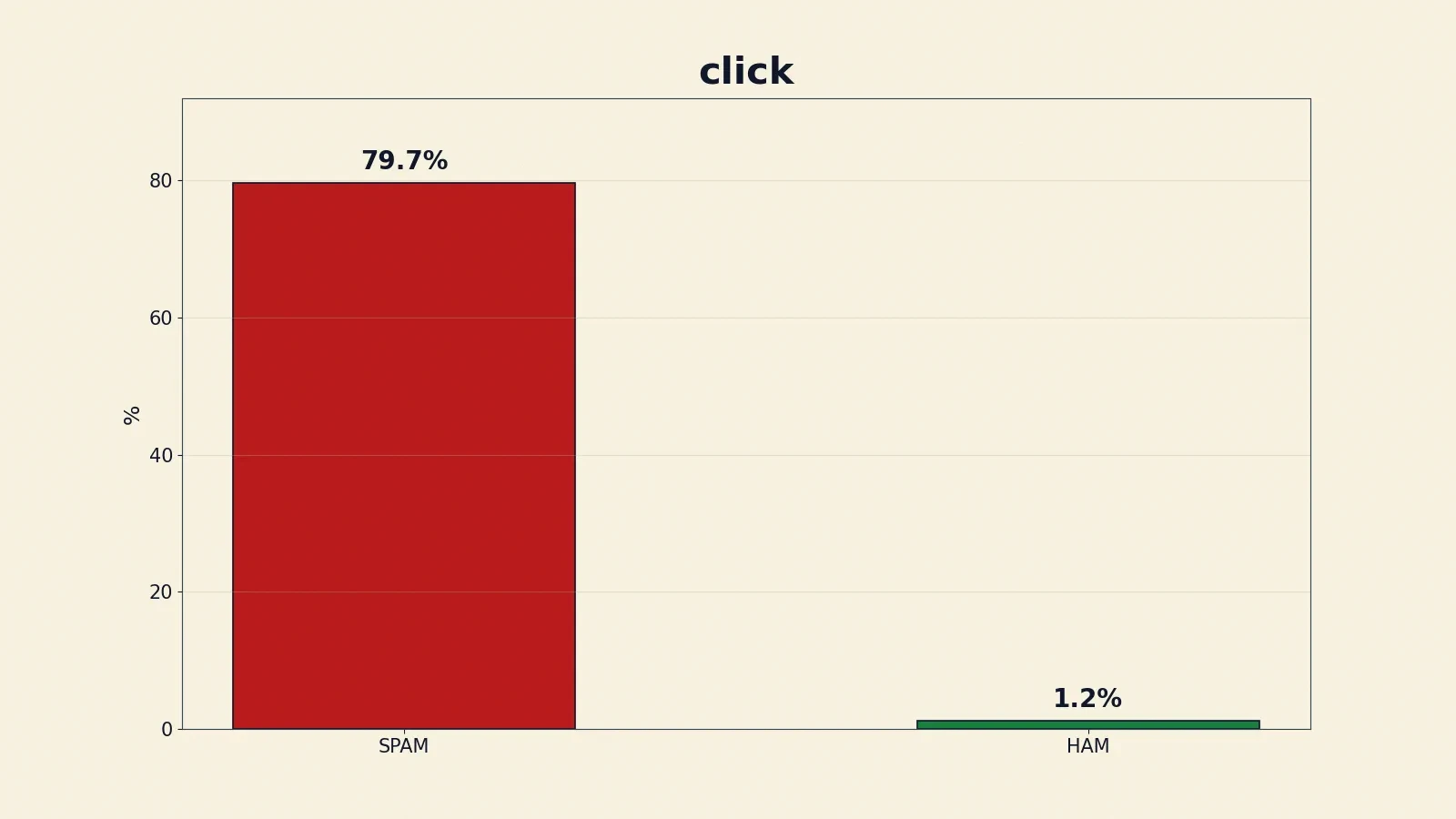
The word "click" alone, in Graham's essay, caught 79.7 percent of his spam corpus with only 1.2 percent false positives. Two words together gave 99.97 percent, under the assumption that the words were independent — an assumption Graham knew was unrealistic, and which the next subsection discusses. The point is not that two words are magic. The point is that each word is a small piece of evidence, with its own likelihood ratio, and Bayes' theorem multiplies them together into a verdict. A word that appears mostly in spam pushes the odds up. A word that appears mostly in ham pushes them down. Fifteen words, each pushing a little, add up to a decision that is usually right.
Graham himself noted that the first papers on Bayesian spam filtering were two papers at the same 1998 conference, by Pantel and Lin and by a Microsoft Research group. Pantel and Lin caught 92 percent of spam with 1.16 percent false positives. In his follow-up work, Graham's own filter caught 99.5 percent of spam with under 0.03 percent false positives. The essay popularised the approach, and variants were soon implemented in DSPAM, SpamAssassin, and SpamBayes. SpamAssassin itself had been first uploaded to SourceForge on 20 April 2001, by Justin Mason, before Graham's essay appeared. Graham did not invent spam filtering. He showed that Bayes' theorem was the right engine for it, and the field followed.
Naive Bayes
The spam filter is an example of a naive Bayes classifier, a family of probabilistic classifiers built directly on Bayes' theorem. It computes the probability of a class given the features as proportional to the prior probability of the class, times the product of the probability of each feature given the class. It assumes that every feature is conditionally independent given the class — that the words in an email, or the symptoms in a patient, carry no information about each other once you know the class. The assumption is almost never literally true. Words do depend on each other. And yet the classifier works remarkably well, trains in a single pass through the data, and remains a standard baseline for text classification: spam, sentiment analysis, topic labelling, news categorisation, support-ticket routing.
Why does a wrong assumption give right answers? Because classification needs a ranking, not a perfect probability. Even when the independence assumption distorts the absolute numbers, it usually distorts them in the same direction for every class, and the ranking survives. The classifier is naive about the world and shrewd about the decision, and the decision is what matters. That is a useful lesson about models in general: a model does not need to be true to be useful. It needs to be useful in the direction you are using it.
Two practical details complete the picture. The classifier needs Laplace smoothing, also called additive smoothing, because a word never seen in the spam training set would otherwise get a probability of zero and veto the whole product. Smoothing gives every word a small non-zero count, so that no single unseen word can overrule all the rest. And real implementations work in log-space, adding log-probabilities instead of multiplying tiny probabilities, to avoid underflow — the problem of numbers so small that a computer rounds them to zero. Both details are bookkeeping, but they are the bookkeeping that turns a classroom formula into a working system.
Finding the USS Scorpion
In May 1968, the American nuclear submarine USS Scorpion, a Skipjack-class boat, was lost with all 99 crew aboard. The cause of the sinking is still unknown. The search for the wreck was led by John Pina Craven, chief scientist of the Navy's Special Projects Office, and it was run as an exercise in Bayesian search theory — a method Craven's team had developed during the search for a hydrogen bomb lost off Palomares in Spain, in January 1966.
The method was disarmingly human. Experts assigned probabilities to nine scenarios for what had happened to the Scorpion, and they bet bottles of Chivas Regal whisky on each scenario, to make their judgments honest. A bet is a prior with consequences: you do not assign a high probability to a scenario you would not put a bottle on. The scenarios were weighted, combined with what was known about the submarine's course and speed, and turned into a probability map of the ocean floor. Search effort was then allocated to the most probable areas first, and the map was updated as each area was searched and found empty. That is sequential Bayesian updating, with ships instead of coin flips: today's posterior is tomorrow's prior, and every empty patch of ocean is evidence.
In late October 1968, the oceanographic research ship Mizar located sections of the Scorpion's hull on the seabed about 400 nautical miles southwest of the Azores, under more than 9,800 feet of water. The betting had worked. Experts placing wagers to reveal honest beliefs is an idea with a flavour of game theory about it — the discipline of designing rules so that people tell the truth — and our Game Theory article explores that flavour in full. Here, the game was simple: put a bottle where your probability is, and the map will be honest.
The Palomares story, which gave Craven's team their method, deserves two sentences of its own. In January 1966, an American B-52 carrying four hydrogen bombs collided with a tanker during refuelling over Palomares, Spain. Craven assigned probabilities to scenarios, weighted them, and the last bomb was located after an 80-day search, in April 1966. The same method, the same discipline: state your beliefs as numbers, bet on them if you want them honest, and update as the search goes on.
Finding Air France Flight 447
The most celebrated modern case of Bayesian search is Air France Flight 447. In the early morning of 1 June 2009, an Airbus A330 flying from Rio de Janeiro to Paris disappeared over the Atlantic with 228 passengers and crew aboard. Two years of search found nothing. In July 2010, the French accident investigation bureau, the BEA, asked a team from the company Metron — Lawrence Stone, Colleen Keller, Thomas Kratzke, and Johan Strumpfer — to produce a probability distribution for the wreck location, accounting for all information about the crash and for the previous search efforts. They used a Bayesian procedure to produce a posterior target location distribution, and the resulting probability map guided the 2011 search.
The wreckage was found on 3 April 2011, after one week of undersea search in the third year, on the ocean bottom about 14,000 feet below the surface, near the centre of the circle in the Metron probability map. The flight data recorder and cockpit voice recorder were then recovered. The paper the team published — Statistical Science, volume 29, pages 69 to 80, DOI 10.1214/13-STS420 — states plainly that failure to use a Bayesian approach in planning the 2010 search delayed the discovery of the wreck. The prior distribution was a mixture of three distributions, and the analysis used a particle filter, a computational method for tracking a distribution as evidence accumulates. The technical details are beyond this article. The moral is not: when you have searched the wrong places for two years, the honest thing to do is to write down everything you know as probabilities, update them with everything you have learned, and search where the map says to search. The Stone and colleagues paper on the search tells the story in full, with the map itself.
One sentence, and no more, on a famous wartime application. Alan Turing used Bayesian reasoning in breaking Germany's Enigma code during the Second World War — the subtitle of McGrayne's history says so plainly, calling Bayes' rule the method that cracked the Enigma code — but the technical details of Turing's methods were not verified for this article, and they are not invented here. The sentence stands as a signpost, not as a history. The spam filter, the submarine, and the airliner are the worked cases. Enigma is the reminder that the same rule was at work, in secret, a generation earlier.
13. Bayesian Versus Frequentist: Two Ways of Thinking About Uncertainty
Bayes' theorem sits at the centre of one of the longest arguments in statistics. There are two schools, the frequentist and the Bayesian, and they disagree about what probability means. This section states the disagreement honestly, and refuses to declare a winner, because the honest comparison is the useful one.
The frequentist view
In the frequentist view, probability is the long-run frequency of an event over many repetitions. A parameter — the unknown chance of a coin landing heads, say — is a fixed but unknown value. The data are random: repeat the experiment, and you get different data. A frequentist 95 percent confidence interval means that if the experiment were repeated many times, 95 percent of the intervals produced would contain the true parameter. It does not mean there is a 95 percent chance the parameter lies in this particular interval. The parameter is fixed. It is either in the interval or it is not, and probability does not apply to it.
The frequentist view is the one most science students are taught first, and it has real virtues. It makes no claims about beliefs, and it needs no prior. It asks a clean question — how often would this result occur by chance, if the experiment were repeated for ever? — and it answers it. The cost is that it never assigns a probability to a hypothesis. It can say how surprising the data would be if a hypothesis were true. It cannot say how likely the hypothesis is, given the data. And the probability of the hypothesis is very often the thing a decision-maker actually wants.
The Bayesian view
In the Bayesian view, probability is a degree of belief. A parameter is an uncertain quantity, described by a probability distribution. The data, once observed, are fixed. A Bayesian 95 percent credible interval means there is a 95 percent probability the parameter lies in this interval, given the data and the prior. That is the sentence most people think a confidence interval means, and it is the sentence the Bayesian interval actually delivers.
The Bayesian view has the opposite virtues and the opposite costs. It gives the probability of the hypothesis, which is what decisions need. It updates cleanly as evidence accumulates. Its cost is the prior: the answer depends on where you started, and a reader who disagrees with your prior will disagree with your posterior. The defence is that the prior is written down, sourced, and open to challenge — and that with a lot of data, Bayesian and frequentist results tend to converge, provided the prior does not rule out plausible values. The disagreement about the prior is a disagreement conducted in the open, with numbers, rather than a disagreement hidden inside a choice of method.
The honest comparison
The draft of this section was nearly written as a contest, with a winner. That would have been a mistake, and the MIT OpenCourseWare reading on the comparison of the two schools, which this section follows, presents both critiques and both defences for a reason. Both approaches evaluate evidence about competing hypotheses. They answer different questions. The frequentist asks how often a procedure would mislead, over infinite repetitions. The Bayesian asks how likely a hypothesis is, given the evidence in hand. A scientist who wants to know whether a result would replicate reaches for the frequentist question. A doctor who wants to know whether this patient has this disease reaches for the Bayesian one.
The table below puts the comparison in one place. Read it across the rows, and notice that every row is the same disagreement, stated four ways.
| Frequentist | Bayesian | |
|---|---|---|
| Parameter | Fixed but unknown value | Uncertain quantity, described by a distribution |
| Probability | Long-run frequency over many repetitions | Degree of belief, updated by evidence |
| Uncertainty | Lives in the data; the parameter is fixed | Lives in the parameter; the data are fixed once observed |
| Prior | No prior; the method needs none | Prior stated openly, then updated to a posterior |
Two cautions close the section. The first is about infinity. The frequentist definition leans on infinite repetitions — what would happen if the experiment were repeated for ever — and that "for ever" is doing real work in the definition. Our Infinity article explores what infinite repetition means and where it breaks down, and it is worth reading before taking the frequentist definition too literally. The second caution is about p-values and confidence intervals, which are among the most misunderstood numbers in science. Our Misleading Statistics article covers that confusion in detail. Read it alongside this section, and the two together give a fuller picture than either alone.
The main critique of Bayesian inference is that a subjective prior is subjective. The main defence is that the probability of a hypothesis is exactly what a decision-maker needs. Both statements are true, and the argument between them has run for two centuries without a victor. That is not a failure. It is a sign that the two schools are answering different questions, and that a working scientist needs both answers, and needs to know which one they are getting.
14. Six Mistakes to Never Make Again (and How to Change Your Mind Correctly)
Everything in this article reduces to six mistakes. Each one has appeared in a classroom, a clinic, or a courtroom. Learn them by name, and you will not make them.
- Confusing P(A|B) with P(B|A). The probability of a positive test given disease is 99 percent. The probability of disease given a positive test is 9 percent. They are different numbers, and confusing them is the single error behind the medical-test surprise, the mammography surprise, and the prosecutor's fallacy. Always ask which way round the conditional runs.
- "A positive test means you almost certainly have it." False when the condition is rare. A 99 percent test at 1 in 1,000 prevalence gives a 9 percent posterior. A positive screen is a reason for follow-up testing, not a diagnosis.
- "Priors are just guesses, so Bayes is subjective and unscientific." False as stated. A prior must be justified — from a measured base rate, from a stated symmetry argument, or from an explicitly declared assumption the reader can inspect and challenge. An unjustified prior is a flaw in the analysis, not in the theorem. Most people assume that using a prior means guessing, but a stated, sourced prior is the most honest part of the calculation.
- "Bayes is magic: feed it anything and it gives the truth." False. Garbage in, garbage out. A wrong prior or a wrong likelihood gives a wrong posterior, however correctly the arithmetic is done. The Sally Clark case is the proof: the arithmetic of squaring was correct, and the independence assumption it rested on was false.
- "A small posterior means the hypothesis is false." False. Nine percent is not zero percent. A positive test at 1 in 1,000 prevalence still raises the chance of disease from 0.1 percent to 9.02 percent — a ninety-fold increase. A small posterior can be a large update, and the size of the update is the measure of the evidence.
- "Bayes' theorem tells you what caused something." It does not. It gives the probability of each candidate cause given the evidence. It cannot create evidence, choose the hypotheses, or justify the prior. The hypotheses come from the world, and from the person asking the question. The theorem only weighs them.
Now return to where this article started. A 99 percent accurate test, a positive result, and a chance of disease of about 9 percent. The same test at a higher prevalence gives 50 percent. An 80 percent reliable witness gives 41 percent. A 90 percent mammogram leaves the chance at 9.2 percent. In every case, the evidence moved the belief, and the prior set the scale. Changing your mind correctly is not about trusting evidence more. It is about weighing evidence against what you already knew.
There is one question to ask before any test result, witness statement, or headline number: how common was this before I saw the evidence? Ask it every time, count the people instead of staring at the percentages, and the theorem will do the rest. Bayes never published his essay, and he never saw the formula that carries his name. He would have recognised the question, though. It is the question his square table was built to answer: given what I have seen, how much should I believe?
Frequently Asked Questions
What is Bayes' theorem in simple terms?
Bayes' theorem is a rule for updating a belief when new evidence arrives. Start with how likely something was before the evidence, weigh how much more often the evidence appears when it is true than when it is false, and you get how likely it is after. It turns a prior and a likelihood into a posterior.
What is an example of Bayes' theorem in real life?
The medical test is the clearest example. A test that is 99 percent accurate is used for a disease found in 1 person in 1,000, and a positive result means only about a 9 percent chance of having the disease. The same test at 1 in 100 prevalence gives exactly 50 percent. The result changes because the base rate changes, not because the test changes.
Why is Bayes' theorem important?
Because it is the correct way to combine what you knew before with new evidence. Without it, rare events are wildly overestimated — in medical testing, in courtrooms, in spam filters, and in search. It is the difference between a test result that frightens a patient needlessly and one that is read correctly.
What is the difference between prior and posterior probability?
The prior is the probability before the evidence, usually the base rate — for example, 1 in 1,000 for the disease in the medical test. The posterior is the probability after the evidence — 9.02 percent after a positive result. The likelihood connects them: it says how much more often the evidence appears when the hypothesis is true.
How do you calculate Bayes' theorem?
Use the formula P(A|B) = P(B|A) x P(A) / P(B), or in odds form, posterior odds = prior odds x likelihood ratio. For the medical test: prior odds 1 to 999, likelihood ratio 99, posterior odds 99 to 999, which converts to 99 divided by 1,098, or 9.02 percent. Counting people in a frequency tree gives the same answer.
Why is a positive medical test often wrong?
Because when a disease is rare, the many healthy people produce more false positives than the few sick people produce true positives. At 1 in 1,000 prevalence, even a 99 percent accurate test gives only a 9 percent posterior. A positive screen is the start of an investigation, and it needs follow-up testing, not panic.
What is the base rate fallacy?
It is ignoring how common something is in a population and judging only by vivid case details. The cab problem is the classic demonstration: 85 percent of cabs are green, 15 percent are blue, and an 80 percent reliable witness says Blue — yet the chance the cab was blue is only 41.4 percent. The witness feels like the evidence. The base rate is doing the work.
What is naive Bayes used for?
Spam filtering above all: Paul Graham's 2002 essay showed how to combine the spam probabilities of individual words with Bayes' rule, and his filter missed fewer than 5 per 1,000 spams with zero false positives. It is also used for sentiment analysis, topic labelling, and text classification. It assumes words are independent given the class, which is false but works well in practice.
Sources
- Principles of Data Science, 3.4 Probability Theory — OpenStax
- Bayesian Epistemology — Stanford Encyclopedia of Philosophy
- Thomas Bayes — MacTutor, University of St Andrews
- Thomas Bayes — Oxford Dictionary of National Biography, via MacTutor
- The True Title of Bayes' Essay — Stephen Stigler, Statistical Science 2013, DOI 10.1214/13-STS438
- An Essay towards solving a Problem in the Doctrine of Chances — Thomas Bayes, 1764, DOI 10.1098/rstl.1763.0053
- Todhunter on Bayes — History of Probability, Chapter 14
- What Did Bayes Really Say? — Kohn, translation and commentary
- Reading 20: Comparison of Frequentist and Bayesian Inference — MIT OpenCourseWare 18.05
- Think Bayes, 2nd edition, Chapter 6: Odds and Addends — Allen Downey
- Think Bayes, Chapter 6: Odds and Addends — Allen Downey
- Module 2.1: Conjugacy, Beta-Bernoulli and Beta-Binomial — Duke STA 360
- Lecture 17: Bayesian Inference, Conjugate Priors — University of Illinois CS 361
- Diagnostic Testing Accuracy: Sensitivity, Specificity, Predictive Values and Likelihood Ratios — StatPearls, NCBI Bookshelf
- Understanding and Using Sensitivity, Specificity and Predictive Values — Parikh et al., PMC
- Natural Frequencies Improve Bayesian Reasoning — Frontiers in Psychology, 2015, DOI 10.3389/fpsyg.2015.01473
- Base Rate Fallacy — Simply Psychology
- Kahneman's Example of Elementary Bayesian Inference — Anesi
- Sally Clark — Wikipedia
- Statement Regarding Statistical Issues in the Sally Clark Case — Royal Statistical Society, 23 October 2001
- R v Sally Clark (2003) — LCCSA
- A Plan for Spam — Paul Graham, August 2002
- Better Bayesian Filtering — Paul Graham, January 2003
- Search for the Wreckage of Air France Flight AF 447 — Stone et al., Statistical Science 2014, DOI 10.1214/13-STS420
- In Search of Air France Flight 447 — INFORMS
- USS Scorpion (SSN-589) — Wikipedia