

On the evening of 3 November 1936, the most famous pollster in America was wrong in front of the whole country, and that night is the best place to begin learning how statistics can mislead. The Literary Digest had mailed about 10 million ballots, collected 2,376,523 replies, and predicted that the Republican challenger Alf Landon would beat President Franklin D. Roosevelt by 57 percent to 43 percent. Hours later Roosevelt won 60.8 percent of the popular vote and carried 46 of the 48 states. The poll had not been small. It had not been careless in the ordinary sense. It had gathered the largest sample anyone had ever taken, and it still missed the result by about 19.6 percentage points. That failure breaks the one belief most of us hold about numbers: that a bigger pile of data must mean a truer answer.
I learned that lesson the uncomfortable way, years before I started writing about numbers for a living. A friend sent me a chart showing that people who drank a particular type of tea lived longer, and I forwarded it to my family the same evening, pleased with myself for sharing something healthy and scientific. A week later I read the small print. The tea drinkers in the study were also younger, richer, and more likely to exercise than the people they were compared with. The chart had not lied about a single number. It had simply left out the one fact that changed what the numbers meant. I had done exactly what the Digest's readers did in 1936: I trusted the size of the evidence and never asked who was missing from it.
This article is a field guide to that kind of mistake. A statistic is a single number computed from data, and statistics is the discipline that produces such numbers. Neither one is the enemy. The danger sits in between the number and the claim made from it: in who was counted and who was left out, in how groups were combined or split, in what was never measured at all, and in how a graph was drawn. The numbers in this article are real, and every worked calculation has been checked twice. The stories come from published research, from a wartime mathematics group, from a hospital study, from a census report, and from two of the most famous polling failures in history. Where a popular retelling gets a detail wrong, this article says so plainly.
1. How Statistics Can Mislead You — Even When Every Number Is True
1.1 The 1936 lesson in one paragraph
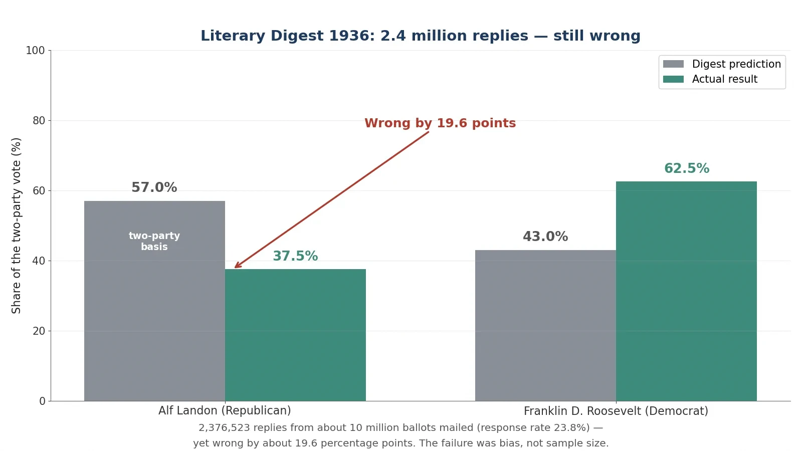
The Literary Digest had correctly predicted the winner of every presidential election from 1916 to 1932, so its 1936 forecast carried enormous authority. It mailed about 10 million ballots drawn from telephone directories, automobile registration lists, club rosters, city directories, and its own subscriber list. Almost 2.4 million came back: 2,376,523 replies, a response rate of 23.8 percent. The prediction, published on 31 October 1936, gave Landon 57 percent against Roosevelt's 43 percent on a two-party basis. The actual result on 3 November gave Roosevelt 60.8 percent of the popular vote to Landon's 36.5 percent, or 62.5 percent to 37.5 percent on the same two-party basis. The Digest was wrong by about 19.6 percentage points, and its margin of error from sampling alone, at a sample of 2,376,523, would have been about plus or minus 0.06 percentage points. The failure was not bad arithmetic. It was bias, and bias does not shrink when the sample grows.
1.2 The difference between a wrong number and a misleading number
A wrong number is a mistake in arithmetic or measurement. Two plus two written as five is a wrong number. A misleading number is usually correct arithmetic built on a crooked foundation. The Digest's count of its own replies was accurate. Its sample was the problem: telephone and car owners in the sixth year of the Great Depression were richer than the country as a whole, and the frame covered only about 60 to 65 percent of adults, missing many of the lower-income voters who leaned Democratic. Only 24 percent of the people who received a ballot replied, and Landon supporters were more likely to send theirs back. About 51 percent of respondents said they had voted Republican in 1932, while only about 40 percent of actual 1932 voters had done so. Every step of the counting was honest. Every step of the choosing was skewed.
That distinction matters because it changes what to check. When a number is wrong, you recheck the arithmetic. When a number is misleading, you have to ask a different set of questions: who was counted, who was left out, what groups were mixed together, what was not measured, and what the chart chose to show. The rest of this article is organised around those questions. Each section takes one classic trick, shows it working in a real case with real numbers, and then gives you the question that exposes it.
There is also a second kind of misleading number worth naming early: the number that is true but answers a different question from the one you think you asked. A fund that reports the average return of the funds still in business is telling the truth about the survivors. It is not telling you the truth about the money people actually put in, because the dead funds are gone from the average. A test that is 99 percent accurate is telling the truth about its own error rate. It is not telling you that a positive result means you are 99 percent likely to be ill, because that depends on how rare the illness is. Keep that gap in mind — the gap between the question the number answers and the question you wanted answered — and most of the tricks in this article become easy to spot.
1.3 The seven tricks this article covers
Seven patterns cover nearly every misleading statistic you will meet in the news, in advertising, or in a meeting room. They overlap, and a single bad chart can use three of them at once, but each has its own shape.
Survivorship bias — counting only the winners that survived long enough to be counted, and forgetting the losers that vanished. Section 2.
Simpson's paradox — a trend in the combined data that reverses inside every subgroup, or the other way round. Section 3.
Correlation mistaken for causation — two things moving together, with no proof that one causes the other. Section 4.
The base rate fallacy — forgetting how rare or common something is before judging a test result. Section 5.
Biased polls and surveys — asking the wrong people, or hearing back only from the keenest. Section 6.
Misleading averages and graphs — picking the average or the picture that flatters the claim. Section 7.
Regression to the mean — mistaking a natural bounce-back from an extreme result for the effect of a treatment. Section 8.
1.4 How to read this article: the sceptic's checklist
Section 9 collects everything into an eight-item checklist you can run on any statistic in under a minute: who is missing from the sample, what the subgroups show, whether the link is causal, what the base rate is, who was asked and who answered, mean or median, where the axis starts, and whether the percentage is relative or absolute. You do not need the checklist to follow the stories. But if you read nothing else, read Section 9. It is the whole article compressed into eight questions, and it is the part I use most often myself when a headline number catches my eye and something about it feels too neat.
The table below is the map. Each row names a trick, what it hides, and where you are most likely to meet it.
Trick | What it hides | Where to spot it |
|---|---|---|
Survivorship bias | The failures that disappeared | Success stories, fund returns, "habits of billionaires" |
Simpson's paradox | The subgroups that point the other way | Admissions, hospital results, league tables |
Correlation vs causation | The third factor driving both | Health headlines, food studies, social trends |
Base rate fallacy | How rare the condition is | Medical tests, screening, security alarms |
Biased polls | Who was never asked, or never answered | Election polls, online surveys, reviews |
Misleading averages and graphs | The skew, the axis, the chosen dates | Income claims, fund charts, bar charts |
Regression to the mean | Luck that will not repeat | Before-and-after claims, extreme cases |
One more warning before the stories begin. Human intuition about numbers is unreliable in a specific way: it treats a precise number as a true number. A forecast of 57.1 percent feels more trustworthy than a forecast of "about half", even when both come from the same flawed sample. Precision is a property of arithmetic, not of truth. The Digest's 57.1 percent was precise to a tenth of a point and wrong by nearly twenty. Hold on to that image as you read. It is the thread that runs through every section that follows.
2. Survivorship Bias: The Planes That Never Came Home
2.1 The bomber problem: Wald, the Statistical Research Group, and the 1943 memos
During World War II the United States military faced a practical problem with a hard limit attached. Bombers were coming home shot full of holes, and the military wanted to add extra armour to protect them. Armour is heavy, and a bomber can only carry so much weight, so the armour could not go everywhere. The question was where to put it so that it saved the most planes. The military took the problem to the Statistical Research Group at Columbia University, a wartime group of mathematicians working at 401 West 118th Street in New York. Its director was W. Allen Wallis, and one of its mathematicians was Abraham Wald, born in 1902 in Kolozsvár, then in the Kingdom of Hungary and now Cluj in Romania.
In 1943 Wald wrote a series of memoranda with a dry title: "A Method of Estimating Plane Vulnerability Based on Damage of Survivors". The title gives away the method. Wald set out a rigorous way to estimate the probability that a hit in each part of an aircraft brings it down, using only the damage recorded on planes that returned. That last phrase is the whole puzzle. The only planes anyone could examine were the ones that had survived. The planes that had been shot down were at the bottom of the sea or scattered across enemy territory, and nobody could count their bullet holes. Wald's job was to draw a conclusion about all the planes from a sample that contained only the lucky ones.
To see how hard that is, try a small toy example, labelled clearly as an illustration and not as history. Suppose 400 planes go out and 380 return, so 20 are lost. That is a loss rate of 20 divided by 400, which is 5 percent. The 380 survivors are the only planes you can inspect. Every hole you see on them is, by definition, a hole a plane can survive. The damage you cannot see — the damage on the 20 lost planes — is exactly the damage you most need to know about. Any conclusion drawn from the survivors alone is a conclusion about survivable damage, not about dangerous damage. That gap is survivorship bias, and it is the single most common way that statistics mislead people who are trying to learn from success.
2.2 Why armouring the holes was the wrong answer
The returning planes showed bullet holes dense on the wings and fuselage and sparse on the engines and cockpit. The obvious proposal was to add armour where the holes were, because that was where the planes were being hit. Wald's point was the opposite. Holes on survivors mark places a plane can be hit and still fly home. The places with few holes on survivors are likely the places where hits were fatal, because those planes never came back to be counted. Armour belongs where the returning planes have no holes: on the engines and the cockpit.
Think of it as a filter. Enemy fire hit planes all over. The planes hit in the wings mostly came home, holes and all, so the wings looked like the most damaged part of the aircraft. The planes hit in the engines mostly did not come home, so the engines looked almost untouched. A count of holes on surviving planes measures the wrong thing. It measures where a plane can afford to be hit. The right question is where a plane cannot afford to be hit, and the survivors cannot answer that question directly, because the answer is written on the planes that are missing. Wald's mathematics filled in the missing planes by reasoning about what the pattern of surviving damage implied about the damage that must have been fatal.
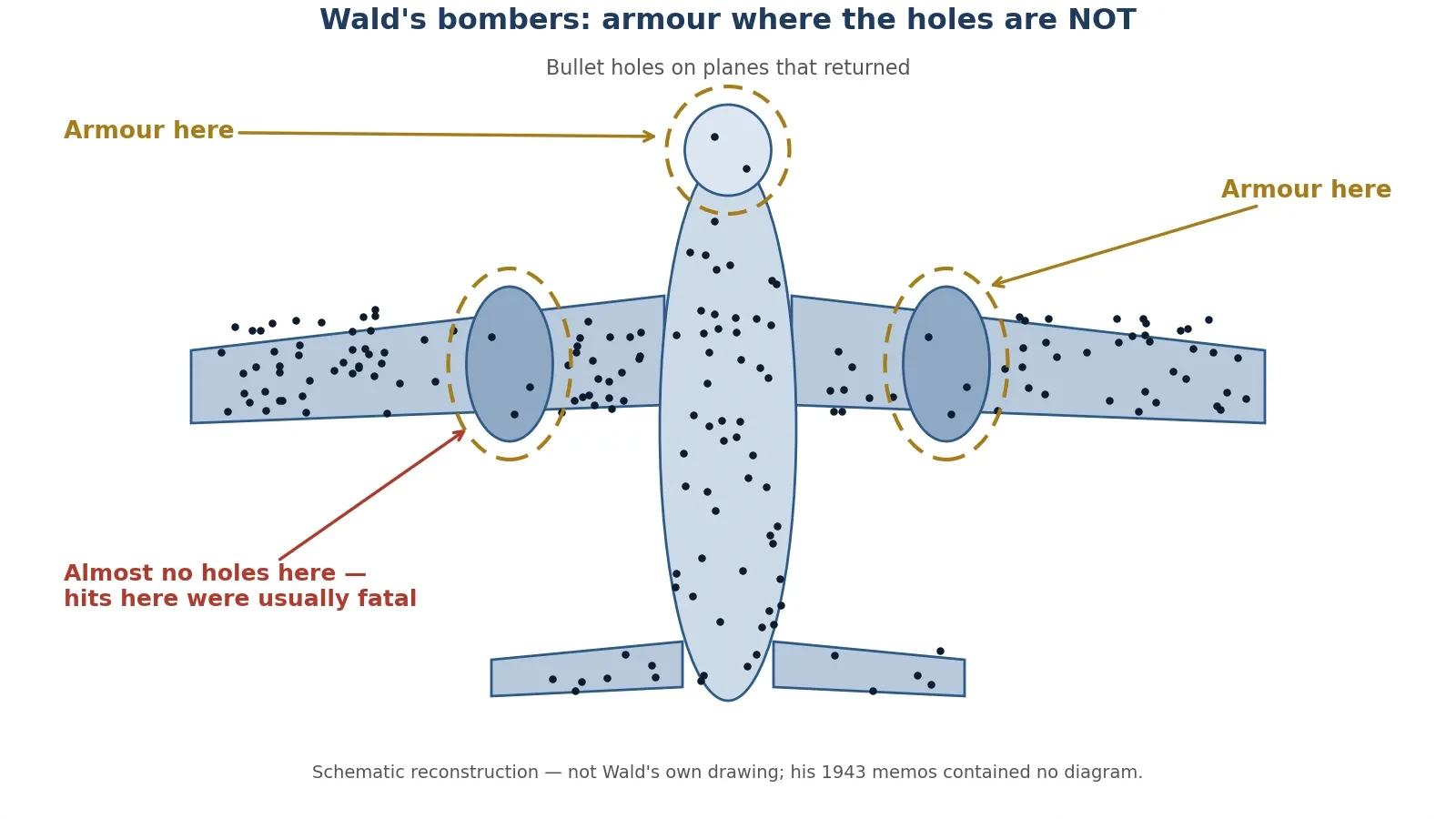
2.3 What the famous story gets wrong
The bomber story is told so often that it has grown details it never had. The honest version is stranger and more interesting than the polished one, so it is worth saying plainly what the popular telling gets wrong. The famous dotted-aeroplane picture was almost certainly never on Wald's desk. The memos contain no aircraft names, and all their worked examples are made up. The diagram is a later reconstruction, loosely based on Wald's 1943 report. There is also no record of sceptical officers in a room, or of a dramatic reversal when Wald spoke up. The two statisticians who studied the memos most closely wrote in 1984 that they did not know whether the method was used during the war at all. The group closed in 1946, and Wald's memos survived because the director took home a box of papers; a colleague at the Center for Naval Analyses published them in 1980.
None of that makes the mathematics less real. Wald's method is genuine, and the logic is sound. But the story should be told as the standard retelling of a real mathematical method, with the diagram labelled as illustrative and the dialogue treated as reconstructed. Presenting the officers scene as documented fact would be exactly the kind of misleading statistic this article warns against: a vivid detail that feels like evidence and is not. One more number to avoid: a modern illustration claims a single hit to the engine was survived 60 percent of the time, against about 95 percent for fuselage and fuel-system hits. That figure comes from an illustration loosely based on Wald's unillustrated report, and it is not a verified Wald number. It does not appear in this article as his.
2.4 The same bias in your money: dead mutual funds vanish from the averages
The bomber problem sounds remote until you look at your own savings. Investment funds publish average returns, and the averages only include the funds that are still alive. A fund that performs badly is usually closed or merged into another fund, and when it disappears it takes its bad record with it. The average that remains is an average of survivors, and it flatters the industry. Carhart, Carpenter, Lynch and Musto measured this in a 2002 study in the Review of Financial Studies and found the annual survivorship bias in average United States mutual-fund performance rises from 0.07 percent for one-year samples to about 1 percent for samples longer than 15 years. The longer the period, the more dead funds have dropped out, and the rosier the surviving average looks. Brown, Goetzmann, Ibbotson and Ross had formalised the problem a decade earlier, in 1992, showing that survivorship can make performance look persistent when it is not.
The scale of the disappearance is large. The S and P Dow Jones Indices SPIVA United States Scorecard for year-end 2024 found that only about 64 percent of United States domestic equity funds that existed 10 years earlier were still operating, and only about 36 percent remained after 20 years. Nearly two-thirds of the funds from twenty years ago are gone. An average computed from the remaining third is not an average of the funds people actually invested in. It is an average of the funds that survived, and the difference between those two averages is the money that vanished quietly. Before trusting any published average return, ask how many funds were in the sample at the start and how many are still there at the end.
2.5 The same bias in success stories
The same filter shapes the advice shelves. A book that promises the ten habits of billionaires studies billionaires. It does not study the far larger number of people who had the same habits and went broke, because those people do not get book deals. A diet book collects the people who lost weight on the diet and stayed slim. It does not collect the people who tried it, regained the weight, and stopped answering the author's emails. A start-up conference invites founders who survived. The founders who failed are not on stage, and their absence makes the survivors' choices look like a recipe instead of a lottery ticket that happened to pay out.
I fell for a version of this myself when I was choosing how to invest a small sum years ago. I read a list of the best-performing funds of the past decade and picked from the top of it, feeling careful and evidence-based. What I had actually read was a list of survivors. The funds that had performed badly for a decade were not on the list, because they no longer existed. My "careful" choice was built on a sample that had already been filtered for success. The list was not lying. It was incomplete in exactly the way the bomber data was incomplete, and I was making exactly the mistake the military nearly made: armouring the holes, and calling it a strategy.
Five everyday places where survivorship bias hides:
Job advice — "I dropped out and became a millionaire" stories never count the dropouts who did not.
Diet books — success stories are collected from people who kept the weight off, not from everyone who tried.
Start-up advice — founders on stage are the ones whose companies lived; the dead companies leave no speakers.
"Old buildings are better built" — the badly built old buildings fell down long ago, so only the good ones remain to admire.
Museum artefacts — the objects that survived centuries are the sturdiest and best-kept, not a fair sample of everything people owned.
3. Simpson's Paradox: When the Total Says the Opposite of the Parts
3.1 What Simpson's paradox is
Simpson's paradox is the most unsettling trick in this article, because it does not need a biased sample or a doctored graph. It needs only a group split into subgroups. A trend present in separate groups disappears or reverses when the groups are combined. The treatment that wins in every subgroup can lose overall. In principle, a group admitted more often in every department can still be admitted less often in total. Edward H. Simpson described the effect in 1951 in a paper called "The Interpretation of Interaction in Contingency Tables", published in the Journal of the Royal Statistical Society, Series B, volume 13, pages 238 to 241. Karl Pearson had noted similar effects in 1899 and Udny Yule in 1903, and the name "Simpson's paradox" was introduced by Colin R. Blyth in 1972. You can read the clearest modern account in the Stanford Encyclopedia of Philosophy entry on Simpson's paradox.
The mechanism is simple once you see it, and it is the same mechanism in every case: the subgroups are different sizes, and the two things being compared are not spread evenly across them. One side gets most of its cases from the easy subgroup. The other side gets most of its cases from the hard subgroup. The overall average is dragged up for the first side and down for the second, even though the second side wins inside every subgroup. The total is not lying. It is answering a different question from the one you think you asked, because it mixes the effect you care about with the effect of who ended up in which group.
3.2 The Berkeley admissions case: 44 percent vs 35 percent overall
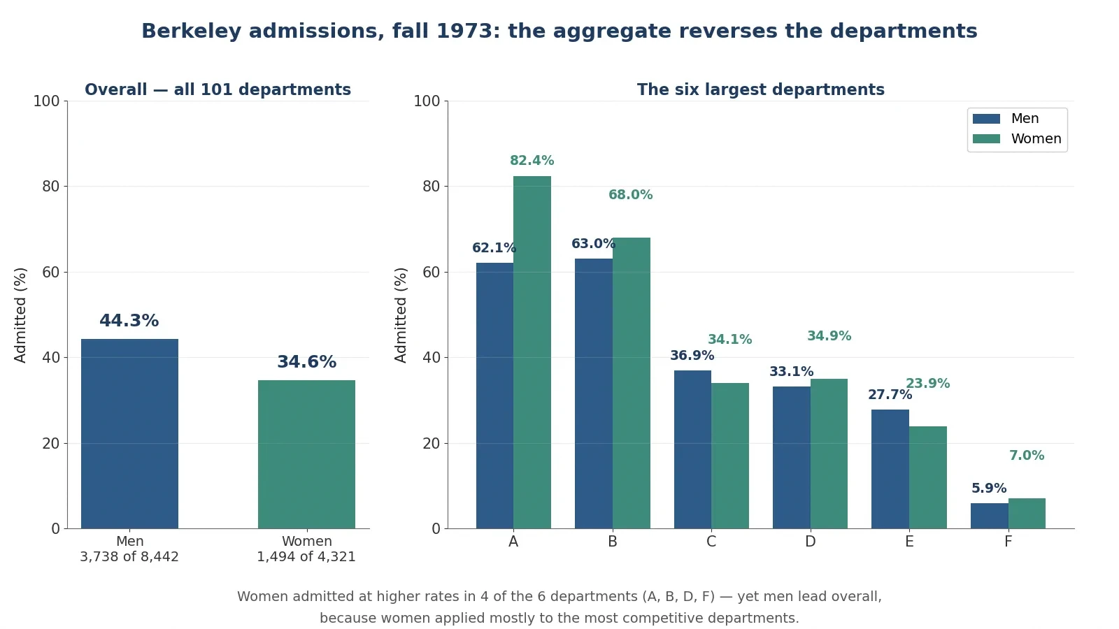
The most famous case comes from the University of California, Berkeley, in the fall of 1973. The Graduate Division received about 15,000 applications, and 12,763 were complete enough for a decision: 8,442 from men and 4,321 from women, across 101 graduate departments. When Peter Bickel, Eugene Hammel and J. W. O'Connell analysed the numbers in a 1975 paper in Science, the aggregate looked like clear evidence of bias against women. Men were admitted at 44.3 percent and women at 34.6 percent. The counts behind those percentages are exact: 3,738 men admitted out of 8,442, and 1,494 women admitted out of 4,321. The gap is 44.28 minus 34.58, which is 9.70 percentage points. In total, 5,232 of 12,763 applicants were admitted, or 40.99 percent. Under no sex effect, the expected admissions would have been 3,460.7 men and 1,771.3 women, so the actual counts differ by 277.3 in each direction: 277 more men and 277 fewer women than expected. The chi-square statistic was 110.8, a value far too large to dismiss as chance.
One detail matters for anyone checking these numbers elsewhere. Several secondary pages state that 1,512 women were admitted. Bickel's Table 1 gives 1,494, with 2,827 rejected, and 1,494 plus 2,827 equals 4,321. The 1,512 figure is inconsistent with the paper's own table and with the 277-person discrepancy. This article uses 1,494 throughout.
A gap of nearly ten points across 12,763 applicants looks like a verdict. It was the starting point of a lawsuit-shaped argument, and it was also wrong as a description of what the departments were doing. The reversal appears when you look department by department.
3.3 Department by department: women admitted at higher rates in 4 of the 6 largest departments
The six largest departments tell a different story. The counts below come from the standard UCBAdmissions dataset drawn from the same paper, and they sum exactly to the published six-department totals: men 1,198 admitted of 2,691, and women 557 admitted of 1,835.
Department | Men admitted | Men rate | Women admitted | Women rate | Who was higher |
|---|---|---|---|---|---|
A | 512 of 825 | 62.1 percent | 89 of 108 | 82.4 percent | Women by 20.3 points |
B | 353 of 560 | 63.0 percent | 17 of 25 | 68.0 percent | Women by 5.0 points |
C | 120 of 325 | 36.9 percent | 202 of 593 | 34.1 percent | Men by 2.9 points |
D | 138 of 417 | 33.1 percent | 131 of 375 | 34.9 percent | Women by 1.8 points |
E | 53 of 191 | 27.7 percent | 94 of 393 | 23.9 percent | Men by 3.8 points |
F | 22 of 373 | 5.9 percent | 24 of 341 | 7.0 percent | Women by 1.1 points |
Six-department total | 1,198 of 2,691 | 44.52 percent | 557 of 1,835 | 30.35 percent | Men overall |
Women were admitted at higher rates in 4 of the 6 departments: A, B, D and F. In department A the gap was enormous, 82.4 percent for women against 62.1 percent for men, a difference of 20.3 points. Yet the six-department totals show men at 44.52 percent and women at 30.35 percent. How can women win in four departments out of six and still lose the total by fourteen points? Because the departments are not equal in size, and the two groups did not apply to them in the same proportions. Department A admitted 62.1 percent of men, and 825 men applied there, the largest male group. Only 108 women applied to department A. Department F admitted only 5.9 percent of men, and 373 men applied there, while 341 women applied. Women were concentrated in the departments with low admission rates, and men were concentrated in the departments with high admission rates. The total mixes the admission rate with the application pattern, and the application pattern wins.
A warning about the two samples is essential. The six-department aggregate for women is 30.4 percent, while the all-department aggregate is 34.6 percent. Some secondary pages quote 44.5 percent against 30.4 percent as "the Berkeley numbers" without saying they cover only the six largest departments. This article labels each number with its sample: 44.3 percent against 34.6 percent is all 101 departments; 44.52 percent against 30.35 percent is the six largest departments only. Mixing the two samples is itself a way of misleading with statistics.
3.4 Why it happened: women applied to the most competitive departments
Bickel and his colleagues found the explanation in the application patterns. Women applied in larger numbers to the most competitive departments, in the humanities and social sciences, where admission rates were low. Men applied more to departments with high admission rates, in engineering and the natural sciences. Across the 101 departments, only a few showed bias, and the number biased toward men roughly equalled the number biased toward women. The paper concluded that the aggregate gap was largely explained by department choice, not by department-level discrimination.
That conclusion needs a careful sentence, because it is easy to overstate. Bickel and his colleagues showed the aggregate gap disappears once department is taken into account. They did not prove no discrimination existed anywhere in the process. What steered women toward the competitive departments in the first place — advice, expectations, earlier schooling, the culture of the fields — is a separate question the numbers do not answer. The honest statement is that the numbers do not show department-level bias. Saying there was no discrimination at all would go beyond the evidence, and going beyond the evidence is the habit this article is trying to break.
The lesson of the Berkeley numbers, in short, is that the aggregate is not the verdict; it is the sum of the verdicts, weighted by who applied where.
3.5 The kidney-stone reversal: the treatment that loses overall but wins in every subgroup
Medicine gives the cleanest demonstration of the same paradox, because the stakes are real and the numbers are exact. Charig, Webb, Payne and Wickham compared treatments for kidney stones in a 1986 study in the British Medical Journal, covering 1,052 patients treated in London hospitals between 1972 and 1985. Of these, 350 had open surgery, 350 had percutaneous nephrolithotomy — PCNL, a form of keyhole surgery — and 328 had extracorporeal shockwave lithotripsy, known as ESWL. Success meant stones eliminated or reduced to under 2 millimetres after three months. You can read the full study in the British Medical Journal paper on PMC.
Overall, PCNL looked better than open surgery. Open surgery succeeded in 273 of 350 cases, or 78 percent. PCNL succeeded in 289 of 350 cases, or 82.6 percent. A reader who stopped there would conclude PCNL was the better treatment. But split the patients by stone size, and the result reverses in both groups. For small stones under 2 centimetres, open surgery succeeded in 81 of 87 cases, or 93.1 percent, against PCNL's 234 of 270, or 86.7 percent. Open surgery wins by 6.4 points. For large stones of 2 centimetres and over, open surgery succeeded in 192 of 263 cases, or 73.0 percent, against PCNL's 55 of 80, or 68.8 percent. Open surgery wins by 4.3 points. Open surgery wins for small stones and wins for large stones, and loses overall. That is Simpson's paradox in a hospital ward.
Group | Open surgery | PCNL | Winner |
|---|---|---|---|
Small stones, under 2 cm | 81 of 87, 93.1 percent | 234 of 270, 86.7 percent | Open surgery by 6.4 points |
Large stones, 2 cm and over | 192 of 263, 73.0 percent | 55 of 80, 68.8 percent | Open surgery by 4.3 points |
Overall | 273 of 350, 78.0 percent | 289 of 350, 82.6 percent | PCNL by 4.6 points |
Two traps hide in this table, and both are worth naming. First, at least one secondary page writes "83 percent (234 of 270)" for PCNL small stones. That is wrong: 234 divided by 270 is 86.7 percent, not 83 percent. The 83 percent figure is PCNL's overall rate, wrongly copied into the small-stone cell. Second, ESWL succeeded in 301 of 328 cases, or 91.8 percent, but it is not part of the paradox comparison and should not be dragged into the reversal table. It was given to a different mix of patients again, and mixing it in would only confuse the comparison.
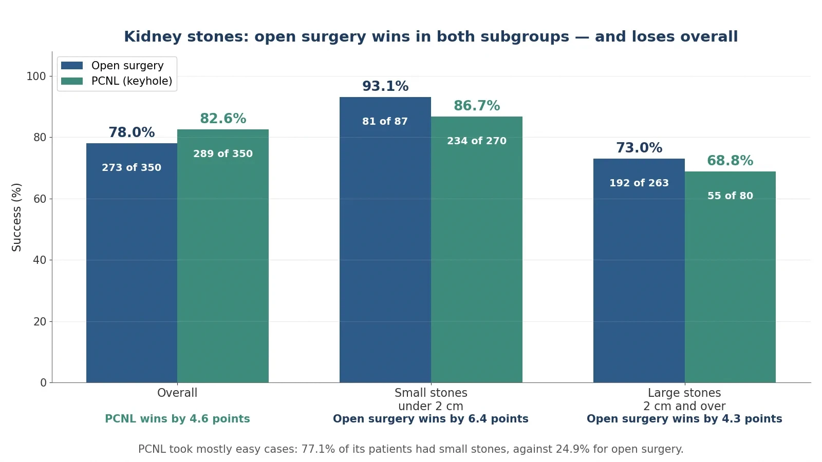
Why did the reversal happen? Doctors avoided open surgery except for the hardest cases. Only 24.9 percent of open-surgery patients, 87 of 350, had small stones, against 77.1 percent of PCNL patients, 270 of 350. PCNL's overall rate is padded with easy cases. Open surgery's overall rate is dragged down by hard cases. The treatment that took the harder patients looks worse in the total, even though it did better with both kinds of patient. This is a historical comparison from 1972 to 1985, not a randomised trial, and that matters: the treatments were given to different kinds of patients, which is exactly why the comparison reverses — and why modern medicine uses randomised trials, where the sorting is done by chance instead of by a doctor's judgement.
3.6 The lesson: always ask what the groups are, and who was sorted into them
Simpson's paradox teaches one question that should become automatic: what are the subgroups, and who was sorted into them? An overall rate is a weighted average, and the weights are the group sizes. Change the weights and the average moves, even when nothing inside any group changes. League tables, hospital rankings, school results, and hiring statistics all run on weighted averages, and all of them can reverse when the groups are examined. The Berkeley case and the kidney-stone case are the two to remember, because they show the same reversal from opposite directions: one about fairness, one about medicine, both about the same arithmetic. Whenever an overall comparison surprises you, split it before you believe it.
4. Correlation Is Not Causation: The Three Ways Two Things Move Together
4.1 The ice-cream-and-drowning story: summer is the hidden third variable
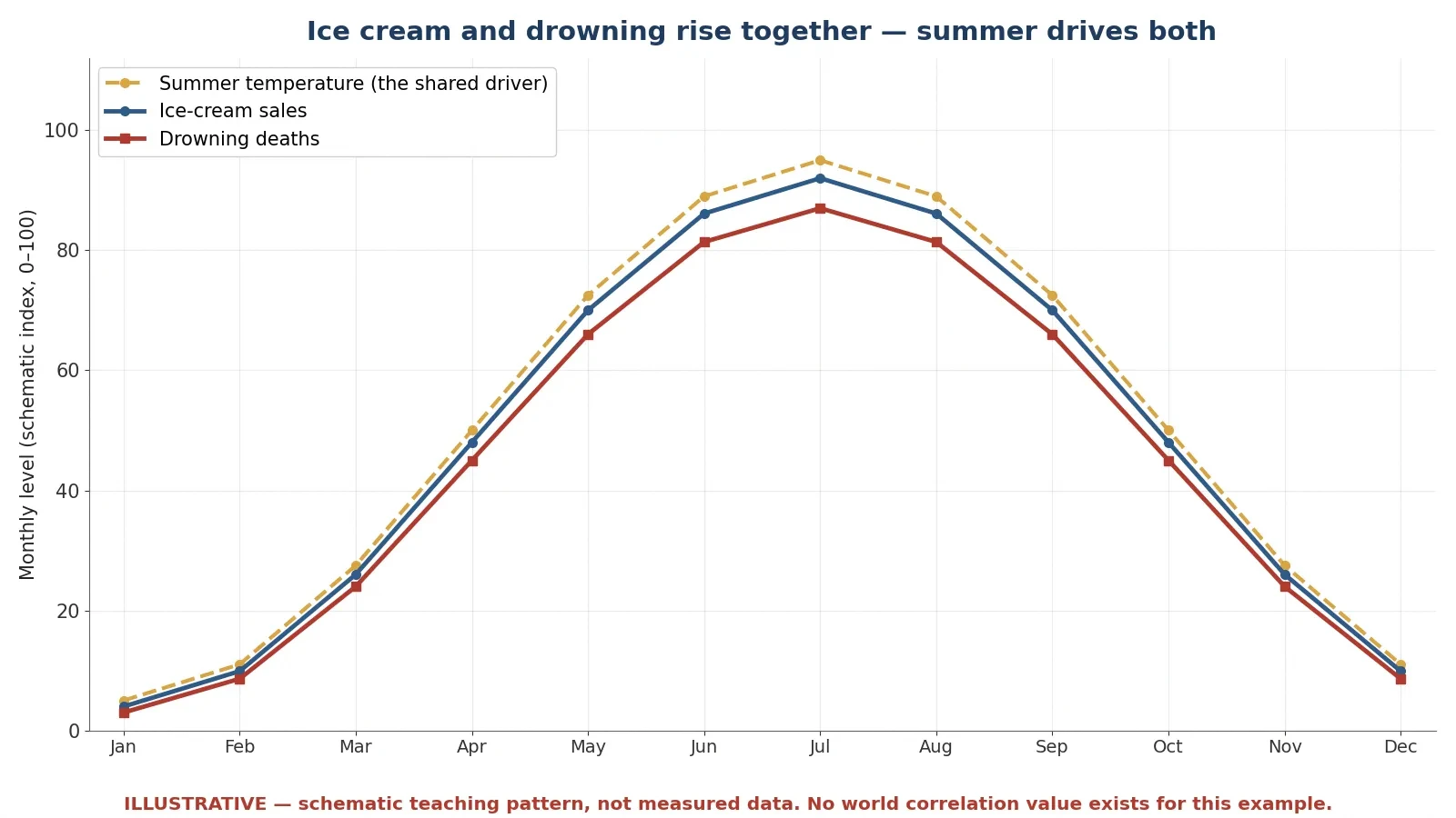
Every statistics textbook tells the same story, and it earns its place because it is so clean. Monthly ice-cream sales and monthly drowning deaths rise and fall together, with a strong positive correlation. When ice-cream sales are high, drownings are high. When sales fall, drownings fall. The pattern is real, and the temptation is to read it as a cause: ice cream causes drowning, perhaps because people swim on a full stomach, or because cold food cramps the muscles. That reading is wrong, and the reason is a third variable that drives both. Hot weather and the summer season drive more ice-cream buying and more swimming, and more swimming means more drownings. Control for temperature and the association disappears.
No single canonical correlation coefficient exists for this example, and honesty requires saying so. Different teaching datasets give different values, and one course text quotes r equals 0.87 for a 12-month teaching dataset — but that is that dataset's number, not a fact about the world. This article does not quote a specific r for ice cream against drowning, because there is no world value to quote. The honest statement is that the correlation is strong and positive, and that it is explained by a shared seasonal cause. A number that looks precise is not automatically a fact, and the ice-cream example is the place to learn that discipline: if a statistic has no named dataset behind it, treat it as an illustration, not as evidence.
The three causal stories to lay out are the same three you should test for every correlation you meet. First, direct causation: ice cream causes drowning. Implausible, and no mechanism survives a moment of thought. Second, reverse causation: drowning causes ice-cream sales. Absurd on its face. Third, confounding: summer causes both. Correct, and the only story that explains why the two rise and fall together through the year. There is a fourth possibility that belongs in every test as well: pure coincidence, which is the subject of the next two sections. A correlation is a clue, not a verdict. It tells you two things move together. It does not tell you why.
4.2 Chocolate and Nobel Prizes: a real NEJM correlation, r = 0.791, that proves nothing
The chocolate story is better than the ice-cream story, because it is real, published, and peer-reviewed — and it still proves nothing about causation. In 2012 Franz H. Messerli published a paper in the New England Journal of Medicine called "Chocolate Consumption, Cognitive Function, and Nobel Laureates", volume 367, number 16, pages 1562 to 1564. Across 23 countries he found a close, significant linear correlation between per-capita chocolate consumption and Nobel laureates per 10 million people: r equals 0.791, with a P value of less than 0.0001. Excluding Sweden, r rises to 0.862. Switzerland led on both measures. Messerli's own arithmetic said about 0.4 kilograms of chocolate per capita per year would be needed to add one Nobel laureate per 10 million people, and for the United States that would be about 125 million kilograms per year. Sweden, he noted, "should" have produced about 14 laureates given its chocolate consumption but had 32 — an outlier he flagged himself. You can read a summary of the paper in the Healio report on Messerli's chocolate study.
"The only possible outlier in Figure 1 seems to be Sweden. Given its per capita chocolate consumption of 6.4 kg per year, we would predict that Sweden should have produced a total of about 14 Nobel laureates, yet we observe 32." — Franz H. Messerli, New England Journal of Medicine, 2012.
The paper is not a joke, and it should not be presented as one. Messerli used Nobel laureates per capita only as a surrogate for population cognitive function because no national cognitive-function data existed, and his reasoning about flavanols in chocolate was a genuine hypothesis. But the paper itself states that the correlation does not prove causation, and it calls for a prospective randomised trial. The author also notes that reverse causation is possible: high cognitive function might stimulate chocolate consumption, rather than the other way round. And this is an ecological correlation — a correlation between country averages — which is especially prone to confounding. Wealth, education, and research spending all track with both chocolate consumption and Nobel prizes. A rich country with strong universities eats more chocolate and wins more Nobels, and the chocolate is the passenger, not the driver. The correlation is real, the numbers are exact, and the causal conclusion is unsupported. That combination is the whole point.
4.3 Nicolas Cage and drowning: r = 0.666 from pure chance, and cheese vs bedsheets at r = 0.947
If chocolate shows that a real correlation can mislead, the next example shows that a strong correlation can mean nothing at all. Tyler Vigen's Spurious Correlations project correlates United States government datasets and reports the pairs that match by chance. The famous pair is the yearly number of people who drowned by falling into a swimming pool against the number of films Nicolas Cage appeared in: r equals 0.666. A companion example from the same site is even stronger: per-capita cheese consumption against deaths by getting tangled in bedsheets, at r equals 0.947 — a higher correlation than most real scientific findings, between two things with no plausible link whatsoever. The spurious correlations write-up reports both pairs, and the numbers are exact for the datasets Vigen used.
Why does this happen? Because Vigen's database holds about 25,237 variables and compares hundreds of millions of pairs. With that many comparisons, strong chance correlations are guaranteed to turn up. A P value under 0.05 means little when millions of tests are run, because 5 percent of millions is still a large number of false alarms. This is data dredging, also called multiple comparisons: if you test enough pairs, some of them will match by luck alone, and the ones that match will look like discoveries. The cheese and bedsheets pair, at 0.947, is stronger than the chocolate and Nobel pair, at 0.791. Strength of correlation is not evidence of a real link. It is evidence that two lines moved together, and with enough pairs to choose from, some lines always will.
4.4 The three causal stories to test every correlation
Most people assume a correlation in a headline is a cause waiting to be named. What the data actually shows, in case after case, is that a correlation is a question waiting to be tested. Run every correlation through four questions before you believe a causal claim about it.
Could A cause B? Is there a plausible mechanism, and does the timing fit — does A come before B?
Could B cause A? Reverse causation is easy to miss, especially when the headline names the direction it prefers.
Could C cause both? Is there a third factor, like summer, wealth, or age, that drives both A and B?
Could it be chance? With enough comparisons, or a small sample, a strong correlation can appear from nothing.
The chocolate case fails on the third question, because wealth and education drive both measures. The Cage case fails on the fourth, because millions of pairs were tested. The ice-cream case fails on the third as well, because summer drives both. Three different examples, three different failures, one test that catches all of them. Readers who want the formal machinery behind this kind of reasoning will find it in the Sciory article on what is probability, which covers conditional probability and Bayes' theorem, and in the article on prime numbers, which shows how easily the human mind finds patterns that are not there.
4.5 Why randomised trials exist: the kidney-stone lesson applied to causation
The kidney-stone study from Section 3 returns here with a second lesson. The doctors who chose open surgery for the hardest cases were not making a mistake. They were doing their jobs, giving the most invasive treatment to the patients who needed it most. But their sensible choices created a comparison that could not be read as a fair test, because the two groups of patients were different from the start. That is the fundamental problem of observational data: the groups were sorted by something, and the sorting is usually connected to the outcome. A randomised trial solves it by sorting with chance. Patients are assigned to treatments by a random process, so the groups start out alike on average — in age, in severity, in wealth, in every factor anyone can measure and every factor nobody thought to measure. The only systematic difference left is the treatment itself.
That is why Messerli called for a prospective randomised trial, and why it is the right answer in principle even when it is impractical in practice. Nobody is going to randomise countries to eat more chocolate for thirty years. But the logic stands: without randomisation, or a convincing substitute for it, a correlation is a starting point for research, not a conclusion. The next time a headline says a food, a habit, or a hobby "causes" something, ask whether the study randomised, or whether it merely watched. Watching can find a correlation. Only a fair comparison can find a cause.
5. The Base Rate Fallacy: Why a 99 Percent Accurate Test Can Be Wrong 91 Percent of the Time
5.1 The worked example, step by step
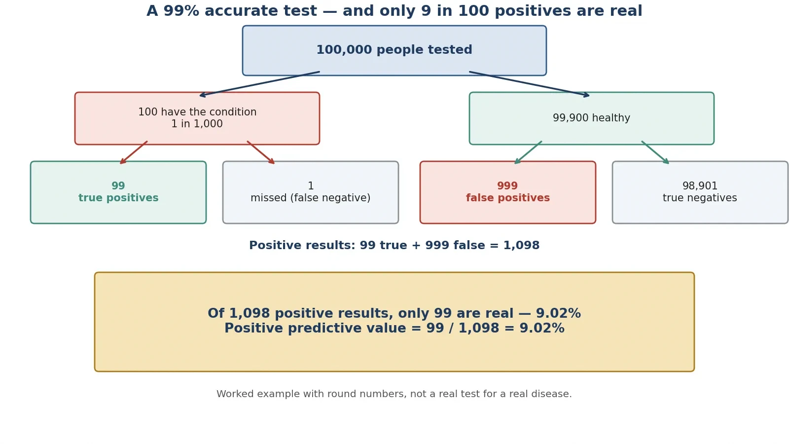
Here is the most counter-intuitive calculation in this article, and it is worth following slowly, because the arithmetic is simple and the result feels impossible. Take a disease that affects 1 person in 1,000. Take a test that is 99 percent sensitive, meaning it catches 99 percent of true cases, and 99 percent specific, meaning it correctly clears 99 percent of healthy people. Apply the test to 100,000 people. This is a worked example with round numbers, not a real test for a real disease. Real tests and real prevalences differ. The point is the arithmetic, which is exact for the stated assumptions.
Start with the population. Diseased: 100,000 multiplied by 0.001 equals 100 people. Healthy: 100,000 minus 100 equals 99,900 people. Now run the test. True positives: 100 multiplied by 0.99 equals 99. False negatives: 100 multiplied by 0.01 equals 1. False positives: 99,900 multiplied by 0.01 equals 999. True negatives: 99,900 multiplied by 0.99 equals 98,901. Total positive results: 99 plus 999 equals 1,098. The positive predictive value — the share of positive results that are true — is 99 divided by 1,098, which is 9.02 percent. A formula cross-check gives the same answer: 0.99 multiplied by 0.001, divided by the sum of 0.99 multiplied by 0.001 and 0.01 multiplied by 0.999, equals 0.0902, or 9.02 percent.
5.2 The answer: only about 9 percent of positives are real
Read that result again, because it is the heart of the section. The test is 99 percent accurate, yet a positive result means only about a 9 percent chance of actually having the disease. About 91.0 percent of positive results are false alarms: 999 divided by 1,098 equals 90.98 percent. The reason is not a flaw in the test. It is the size of the healthy population. The disease is rare, so the healthy group is enormous — 99,900 people against 100. Even a 1 percent error rate in that enormous group produces ten times more false positives, 999, than the true positives, 99, that the disease itself produces. The test's accuracy and the result's trustworthiness are two different numbers, and the gap between them is the base rate: how common the condition is before testing.
The 2-by-2 table below lays out the same arithmetic in the standard form. Sensitivity is the true-positive rate. Specificity is the true-negative rate. Positive predictive value is the share of positive results that are true.
Has the disease (100) | Healthy (99,900) | Total | |
|---|---|---|---|
Test positive | 99 true positives | 999 false positives | 1,098 |
Test negative | 1 false negative | 98,901 true negatives | 98,902 |
Total | 100 | 99,900 | 100,000 |
5.3 Why your brain gets it wrong
We hear "99 percent accurate" and our minds substitute a simpler claim: a positive result is 99 percent certain. That substitution feels natural because it confuses two different conditional probabilities. The test is right 99 percent of the time when the person is diseased, and right 99 percent of the time when the person is healthy. But the question a person with a positive result actually asks is the reverse: given that the test is positive, how likely am I to be diseased? That question depends on how many diseased and healthy people were tested in the first place, and when the disease is rare, the healthy people dominate the answer. Bayes' theorem is the formal machinery that turns the first question into the second, and readers who want the full treatment will find it in the Sciory article on what is probability. The algebra of Bayes' theorem itself is explained step by step in the article on how algebra works.
I made this mistake myself, in a small way, the first time a routine screening result came back flagged. The letter said the test was highly accurate, and for about an hour I walked around believing the flag meant near-certainty. Then I did the arithmetic on the back of an envelope, with the prevalence of the condition written at the top, and the 9 percent figure stared back at me. The follow-up test was negative. The lesson stayed with me longer than the worry did: accuracy is a property of the test, and certainty is a property of the test plus the base rate. A test result without a base rate is a numerator without a denominator.
5.4 Where this bites in real life
The same arithmetic bites wherever a rare condition is screened in a large population. Screening programmes for rare diseases face it by design: test a million healthy people with a 99 percent specific test and you get 10,000 false alarms for every small number of true cases, which is why screening is usually aimed at groups where the condition is more common, and why a positive screening result is followed by a second, different test rather than by treatment. Spam filters face it too: genuine spam is common enough that the base rate helps, but a filter tuned to catch nearly all spam will also flag some ordinary mail, and the cost of those false alarms shapes how aggressive the filter can be. Airport security alarms face it in the extreme: the thing being screened for is vanishingly rare, so almost every alarm is a false one, and the system is designed around that fact, with human checks as the second stage. Keep to the general principle here, and never invent a disease-specific claim: the point is the arithmetic, which is the same in every case. Three questions to ask about any positive test result:
How common is the condition? The rarer it is, the more false positives dominate.
How often does the test cry wolf? A 1 percent false-positive rate is small for one person and enormous across a large population.
What happens next? A positive result should trigger a confirmatory test, not a conclusion.
6. Polls and Surveys: Why 2.4 Million People Can Be Wrong and 50,000 Can Be Right
6.1 The Literary Digest disaster of 1936, told in full
The Digest's failure deserves a full telling, because it is the largest polling error in history measured against the largest sample ever taken. The magazine had correctly predicted the winner of every presidential election from 1916 to 1932 with its straw polls, and for 1936 it mailed about 10 million ballots, drawn from telephone directories, automobile registration lists, club rosters, city directories, and its own subscriber list. Almost 2.4 million were returned: the exact figure cited in the literature is 2,376,523, a response rate of 23.8 percent. The prediction, published on 31 October 1936, five days before the election, gave Republican Alf Landon 57 percent against Democrat Franklin D. Roosevelt's 43 percent on a two-party basis. With third-party candidate William Lemke included in the denominator, the figure was 54 percent for Landon. The final returned counts were Landon 1,293,669 and Roosevelt 972,897, and 1,293,669 divided by the sum of 1,293,669 and 972,897 is 57.1 percent.
The actual result on 3 November 1936 was Roosevelt 60.8 percent of the popular vote to Landon's 36.5 percent, carrying 46 of 48 states — Landon took only Maine and Vermont — and 523 electoral votes to 8. On a two-party basis Roosevelt took 62.5 percent and Landon 37.5 percent. On the like-for-like two-party basis, the Digest put Landon at 57 percent against an actual 37.5 percent, an error of about 19.6 percentage points. The magazine's credibility was destroyed. It folded in 1938, sold that year and shortly after dissolved into Time. A poll with 2,376,523 replies had been beaten by a poll with about 50,000, and the reason is the subject of the next two sections.
6.2 Two biases, not one: coverage bias and nonresponse bias
The Digest failed through two reinforcing biases, and scholars still debate which mattered more, so this article does not declare one the sole cause. The first was coverage bias, also called selection bias. The sampling frame — telephone and car owners — systematically excluded lower-income Americans in the sixth year of the Great Depression. The frame covered roughly 60 to 65 percent of adults, and the uncovered 35 to 40 percent leaned Democratic. The sample was not a cross-section of the country. It was a cross-section of the part of the country that owned phones and cars.
The second was nonresponse bias. Only 24 percent replied, and Landon supporters were more likely to return their ballots. The evidence is in the respondents' own history: about 51 percent of respondents said they had voted Republican in 1932, while only about 40 percent of actual 1932 voters had done so. The people who answered were not like the people who did not answer, and the difference ran in the same direction as the coverage bias. Both biases pushed the result toward Landon, and together they overwhelmed a sample of 2.4 million. Gallup, writing in 1938, blamed the frame. Bryson, in 1976, argued nonresponse was the main cause. Lohr, in 2017, showed that weighting the poll's own 1932-vote data would have predicted a Roosevelt win. A 2012 reanalysis by Lusinchi, using Gallup's 1937 survey data, found that phone and car owners themselves favoured Roosevelt, at 53.9 percent, and put most of the error — 13.7 of the 19.6 points — on nonresponse rather than on the frame, which cost 5.9 points; Squire, in 1988, had given the frame a larger share. The honest summary is that both biases were present and both pointed the same way.
6.3 Gallup's 50,000: quota sampling beats a giant biased sample
George Gallup's American Institute of Public Opinion, founded in 1935, used quota sampling: interviewers were given quotas for age, sex, region, and other characteristics, so the sample was built to match the population instead of merely being large. His final forecast, published on 2 November 1936, gave Roosevelt 55.7 percent of the two-party vote. He called the right winner, from a sample of about 50,000 respondents, drawn from 312,551 ballots sent out. But he was not nearly exact, and the retellings that say so are wrong. Against Roosevelt's actual 62.5 percent two-party share, Gallup's 55.7 percent was 6.8 points low. Many retellings say Gallup predicted 56 percent for Roosevelt and call him nearly exact. The precise two-party figure is 55.7 percent, and the like-for-like error is 6.8 points, not near-zero.
Gallup did something else that year that is often misreported. From a 3,000-person pilot drawn from the Digest's own lists, he predicted in advance that the Digest would find Landon 56 percent to Roosevelt 44 percent — within a point of the Digest's actual 57 to 43. That 3,000 figure is the pilot predicting the Digest's result, not the sample of his election poll. Do not say Gallup predicted the election from 3,000 people. He predicted the Digest's error from 3,000 people, and he predicted the election from about 50,000. The contrast stands either way: 50,000 people chosen to match the population beat 2,376,523 people chosen from phone books. Size is not representativeness, and no amount of size can fix a sample that never had a chance of looking like the country.
6.4 2016: the national polls were right and the state polls missed
Eighty years later, the same lesson returned in a subtler form. An evaluation of the 2016 United States election polls by an ad-hoc committee of the American Association for Public Opinion Research, chaired by Courtney Kennedy of the Pew Research Center, found that the national polls were generally correct and accurate by historical standards. They collectively put Clinton about 3 points ahead. She won the popular vote by 2.1 points, an average absolute error of 2.2 points on the margin, among the most accurate national polling since 1936. The national polls were fine. The state polls were the problem.
State polls had an average absolute error of 5.1 points on the margin, with a signed error of 3.0 points toward Clinton. In the 13 states decided by 5 points or fewer, polls underestimated Trump's margin by 2.3 points. Wisconsin polls underestimated Trump by 6.5 points, Ohio by 5.2 points, Pennsylvania and Minnesota by 4 to 5 points, Michigan by about 3.5 points, North Carolina by more than 4 points, and New Hampshire by more than 3 points. State polls named the wrong winner in Pennsylvania, Michigan, and Wisconsin — the three states that decided the Electoral College. The report's best-supported causes were late-deciding voters, with about 13 percent of voters in Wisconsin, Florida, and Pennsylvania deciding in the final week and breaking heavily for Trump, and a failure to weight by education, because education tracked vote choice closely and better-educated people answer surveys more readily. The report did not find evidence for a "shy Trump voter" effect as a main cause. You can read the Pew summary in the Pew Research questions and answers on 2016 polling.
The 2016 lesson is the mirror image of 1936 in one respect and the same in another. The national polls were fine and the state polls missed, which is the opposite pattern from 1936, when the giant national poll failed. But in both elections the error came from who was reached and who answered, not from the mathematics of sampling error. The maths was sound in both cases. The sample was the problem in both cases.
6.5 Margin of error, honestly explained
The margin of error is the most quoted and most misunderstood number in polling. It measures random sampling error only: how far a result from a random sample might sit from the true value by chance. It says nothing about bias. The formula, at 95 percent confidence and worst case, where p equals 0.5, is 1.96 multiplied by the square root of p multiplied by 1 minus p, divided by n. The table below gives the results, computed in Python, for the sample sizes that matter in this article.
Sample size (n) | Margin of error, 95 percent confidence |
|---|---|
400 | plus or minus 4.90 percentage points |
1,000 | plus or minus 3.10 percentage points |
10,000 | plus or minus 0.98 percentage points |
50,000 (Gallup 1936 scale) | plus or minus 0.44 percentage points |
2,376,523 (Literary Digest 1936) | plus or minus 0.06 percentage points |
Two lessons follow. First, the returns diminish fast. Quadrupling the sample only halves the margin of error: 400 to 1,600 would cut 4.9 to about 2.45. That is why serious polls stop around 1,000 to 2,000 respondents. Going from 1,000 to 10,000 buys only about two more points of precision, and going from 10,000 to 2.4 million buys less than one. Second, the Digest's margin of error was 0.06 points and it missed by 19.6 points — more than three hundred times its own margin. That is not a sampling failure. It is proof that the margin of error never covered the real risk, which was bias. Always state the confidence level, 95 percent here, and remember the formula assumes a random sample with p equal to 0.5, the maximum-variance case. Real polls report slightly different margins because their p differs from 0.5 and they adjust for design effects. Five questions to ask about any poll:
Who was sampled? A random sample of the whole population, or a convenient slice of it?
How were they reached? Phones, cars, the internet, and doorsteps each reach different people.
Who answered? A 24 percent response rate means three-quarters of the sample is unknown.
When was it taken? Late deciders can move a close race in the final week.
What is the margin of error — and the likely bias? The first is printed. The second is the one that decides elections.
7. Averages That Lie and Graphs That Cheat
7.1 Mean vs median: US household income 2025
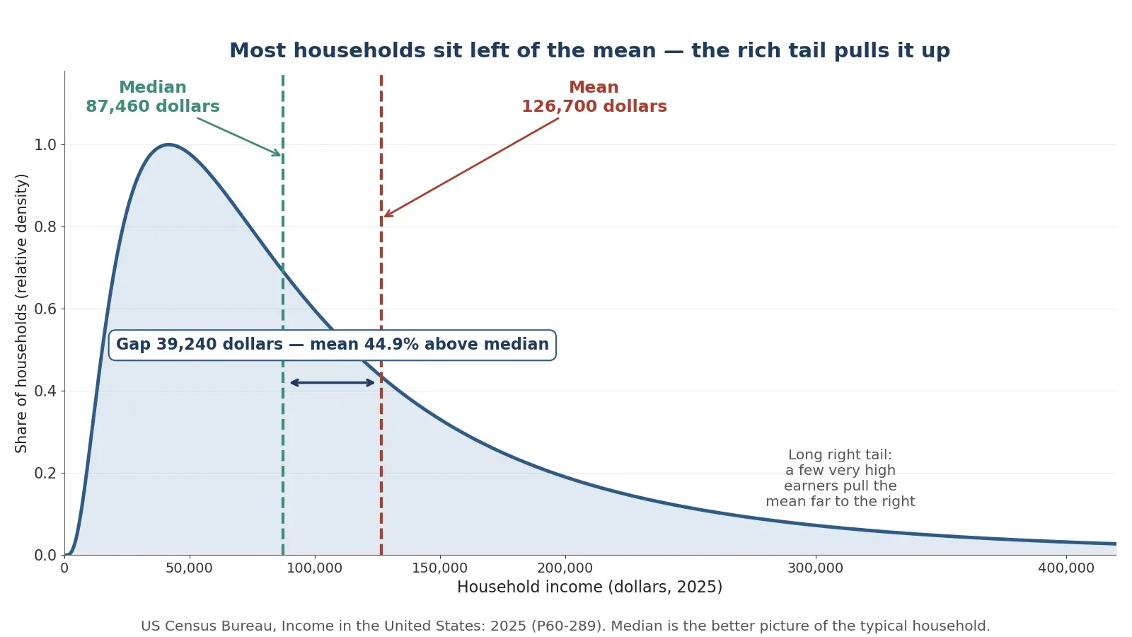
The word "average" hides a choice, and the choice changes the answer. The United States Census Bureau's report "Income in the United States: 2025", issued in September 2026, gives both numbers for household income in 2025 dollars, and the gap between them is the story. Median household income in 2025 was 87,460 dollars, up 2.6 percent from the revised 2024 figure of 85,210 dollars, and the highest on record since the series began in 1967. Mean household income in 2025 was 126,700 dollars. The gap is 126,700 minus 87,460, which is 39,240 dollars. The mean sits 44.9 percent above the median: 39,240 divided by 87,460 equals 0.4487. The Census Bureau story on median household income reports both figures.
Which number describes "the typical household"? The median. The median is the middle value: half of households earn more and half earn less. The mean is the total divided by the number of households, and a small number of very high earners pull it up. When a headline says "the average American household earns 126,700 dollars", it is using the mean, and it is describing a household that earns far more than most households actually do. The median household earns 87,460 dollars. The difference is not a rounding error. It is 39,240 dollars, and it is the difference between a typical household and a statistical artefact. For context from the same report, the post-tax median was 76,060 dollars in 2025, up 3.1 percent from 73,760 dollars in 2024.
One caution about the 2024 median, for readers checking other sources. The 2024 median has two published values: the original September 2025 release put it at 83,730 dollars in 2024 dollars, while the September 2026 release revised the 2024 figure to 85,210 dollars in 2025 dollars, using new population estimates in a different dollar year. This article uses one consistent vintage, the 2025 pair above, and does not mix 83,730 with 126,700. Mixing vintages is a quiet way of manufacturing a trend that does not exist.
7.2 The nine-household toy example
A small invented example makes the mechanism visible. Take nine households with annual incomes of 45,000, 52,000, 58,000, 61,000, 65,000, 70,000, 78,000, 85,000, and 900,000 dollars. The mean is 1,414,000 divided by 9, which is 157,111 dollars. The median is 65,000 dollars, the fifth of nine sorted values. Now remove the 900,000-dollar household. The mean of the other eight is 514,000 divided by 8, which is 64,250 dollars — almost identical to the median. One extreme earner more than doubles the mean while the median barely notices. This is an invented illustration with round numbers, labelled as such, and it shows exactly why income is always reported with a median: income distributions have a long right tail, a small number of very high earners, and the mean follows the tail while the median follows the middle. Whenever a distribution is skewed — income, house prices, company sizes, waiting times — ask for the median. The mean answers a different question: what the total would be if it were shared equally, which is rarely the question anyone is asking.
7.3 Truncated axes: why bar charts must start at zero
A bar chart is read by length. The eye compares the height of one bar with the height of another, and the brain treats the ratio of the lengths as the ratio of the values. That reading is only honest when the bars start at zero. If a y-axis starts just below the data, a 2 percent change can look like a doubling, because the visible part of the taller bar is twice the visible part of the shorter one even though the values differ by almost nothing. The chart has not changed a single number. It has changed the lengths, and the lengths are what the reader actually judges.
Line charts are different. A line chart is read by slope and by change, and a narrowed axis can be honest there, provided the truncation is labelled clearly so the reader knows the axis does not start at zero. The rule is simple to state and easy to apply: bar charts must start at zero because readers judge by bar length; a y-axis that starts just below the data can make a small change look enormous. When you see a bar chart with a broken or shortened axis, mentally redraw it from zero before you believe the comparison. If the difference vanishes when you do, the difference was in the drawing, not in the data.
7.4 Cherry-picked time ranges: the S and P 500 from peak, trough, and recovery
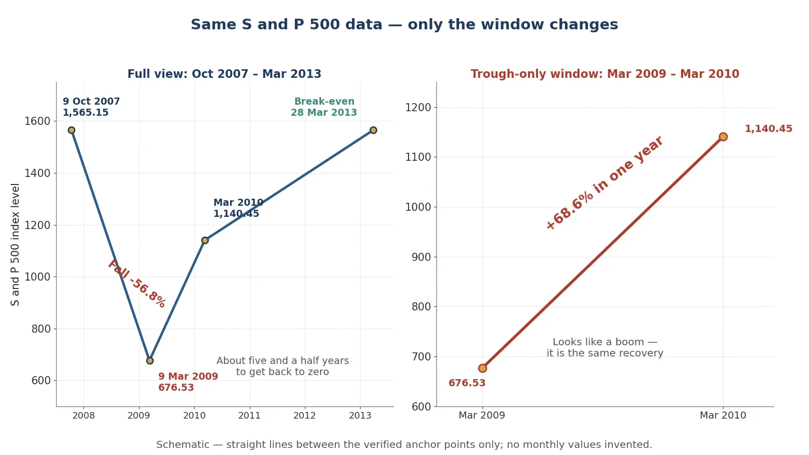
Choosing where a chart starts is choosing what story it tells, and the S and P 500 across the financial crisis shows it with real numbers. The index closed at 1,565.15 on 9 October 2007 and at 676.53 on 9 March 2009: a fall of 56.8 percent, since 676.53 minus 1,565.15, divided by 1,565.15, equals minus 0.5678. It did not close above its 2007 high again until 28 March 2013. Twelve months after the trough it stood at 1,140.45, a rise of 68.6 percent from the low, since 1,140.45 minus 676.53, divided by 676.53, equals 0.6857.
Three charts from the same index tell three stories. A chart starting at the March 2009 trough shows a near-69 percent surge in a year: "the market soared". A chart starting at the October 2007 peak shows a 57 percent collapse: "the market crashed". A chart from peak to recovery, 2007 to 2013, shows five and a half years to get back to zero. All three use the same real index. Only the window changes. Starting a performance chart at a trough flatters returns, and starting at a peak does the reverse. A portfolio described as performing "since 2009" looks heroic precisely because 2009 was the bottom of the financial crisis. The honest chart shows the full period, peak to trough to recovery, and lets the reader see which part of the story the window was chosen to hide.
The question to ask about any performance chart is the same one you ask about any statistic: why does it start when it starts? A chart that starts at a round date — the start of a decade, the start of a fund's life — is making a neutral choice. A chart that starts at a market low, a crisis, or the day a policy changed is making an argument. The starting date is a claim, and it should be read as one. The same habit applies to rates of change more generally: how fast something is rising depends on where you start measuring, and the Sciory article on how calculus works explains rates of change, and how easily a steep-looking slope can be an artefact of a short window.
7.5 Lies with percentages: relative vs absolute risk
Percentages are the most flexible tool in the misleading-statistics kit, because a percentage without its base rate is a sentence without a subject. Take a worked example with round numbers, labelled as illustrative and not a real drug. A trial finds the risk of an event falls from 2 percent without the drug to 1 percent with it. The relative risk reduction is 0.02 minus 0.01, divided by 0.02, which is 50 percent. The headline writes itself: "Drug cuts risk by half!" The absolute risk reduction is 0.02 minus 0.01, which is 1 percentage point. Per 1,000 people, that is 20 events without the drug against 10 with it, and 990 of 1,000 untreated people and 980 of 1,000 treated people never have the event anyway. The number needed to treat is 1 divided by 0.01, which is 100: one hundred people must take the drug for one person to benefit.
Measure | Per 100 people | Per 1,000 people |
|---|---|---|
Events without the drug | 2 | 20 |
Events with the drug | 1 | 10 |
Absolute risk reduction | 1 person in 100 | 10 people in 1,000 |
Relative risk reduction | 50 percent | 50 percent |
Number needed to treat | 100 | 100 |
Both numbers are true, and they describe the same trial. The honest sentence gives both: "Risk falls from 2 in 100 to 1 in 100 — a 50 percent relative cut, but only 1 extra person in 100 helped." A headline that gives only the relative figure is not lying. It is choosing the number that sounds largest, and leaving the reader to imagine a benefit far bigger than the trial found. Two related traps belong in the same paragraph. "Increased by 200 percent" means tripled, because a 100 percent increase doubles the original. And "three times more likely" is ambiguous in ordinary speech, so always state the base rate alongside any percentage change. A percentage is a fraction, and a fraction without its denominator is not information. It is decoration.
8. Regression to the Mean: Why the Worst Always "Improves"
8.1 Galton 1886: 205 families, 930 children
Francis Galton published the founding study of regression to the mean in 1886, in a paper called "Regression towards mediocrity in hereditary stature", in the Journal of the Anthropological Institute, volume 15, pages 246 to 263. Galton measured 205 families with 930 adult children, and he found that children of tall parents were tall but, on average, only about two-thirds as far above the population average as their parents. Parents 3 inches above average had children about 2 inches above average. The population average in his data was about 68.25 inches, or about 173 centimetres. The arithmetic is simple: 3 multiplied by two-thirds equals 2.0 inches, and 5 multiplied by two-thirds equals 3.33 inches. A fitted regression slope of about 0.65 on centred data is reported for the Galton dataset, with an intercept of about 68.09 inches at the population mean.
8.2 The mechanism: extreme results are part luck, and luck does not repeat
An extreme measurement is usually a mixture of a real underlying value and luck. A very tall parent is tall partly by inheritance and partly by the luck of nutrition, health, and chance in development. The children inherit the underlying tendency but not the luck, so they land closer to the average. The same logic holds for a test score, a sales month, a sporting performance, or a hospital's death rate in a single year. The most extreme results contain the most luck, and luck does not repeat. Measure the same people again and the extremes move back toward the average, not because anything changed, but because the lucky part of the first measurement was never going to happen twice.
8.3 The trap in real life
This is why the "worst" schools, hospitals, or players "improve" after an intervention that did nothing, and why praising or punishing an extreme result and then watching it moderate is not evidence the praise or punishment worked. Pick the worst performers, do something — anything — and measure them again. They will have improved, on average, because their first measurement contained bad luck that has now washed out. Pick the best performers and praise them, and they will have worsened, on average, for the same reason. The classic applied warning is never to judge a treatment by before-and-after change in the most extreme cases alone. A diet tested only on people at their heaviest, a training method tested only on players in a slump, a policy aimed only at the worst schools: all three will show improvement even if the intervention is useless, because regression to the mean was always going to do the work.
I watched this happen in a small way with a friend who runs a local sports team. After a dreadful run of results he changed the training routine, and the team promptly won three games in a row. He was convinced the new routine had fixed everything, and he told everyone so. I pointed out that the dreadful run had been the worst stretch in the team's history, and that a team that bad by luck was likely to improve whatever he changed. He laughed, and then he kept the routine anyway, which was fair enough — the routine might have helped. But the three wins were not evidence that it had. They were evidence that extremes do not last.
8.4 What regression to the mean is NOT
One misunderstanding deserves a firm correction, because it is the most common one. Regression to the mean does not mean the population becomes more average over generations. The variance stays. Tall parents still have tall children, and the spread of heights in the population does not shrink. Only the prediction from a selected extreme shrinks: if you select parents who are 3 inches above average, you predict their children at about 2 inches above average, but the children themselves still vary widely around that prediction. The population keeps its shape. The selected group moves back toward the middle. Confusing the two is how people end up believing that excellence is being bred out of a population, or that a policy has narrowed inequality, when all that happened was a statistical bounce.
9. How Statistics Can Mislead You — And How to Talk Back to a Statistic
9.1 The sceptic's checklist
Everything in this article compresses into eight questions. Run them on any statistic — a headline, a chart, a poll, a trial result — and most misleading numbers will fail at least one of them. Keep the list somewhere you can reach it. I keep a version of it on a card by my desk, and I still catch myself skipping a question when a number confirms something I already believe.
Who is missing from the sample? The planes that never came home, the funds that closed, the people who never answered. If the missing group differs from the counted group, the number is a number about the counted group only.
What are the subgroups? Split the total before you believe it. Berkeley and the kidney-stone study both reversed when split, and the split is where the truth lives.
Correlation or causation — and which direction? Test all four stories: A causes B, B causes A, C causes both, or pure chance.
What is the base rate? A 99 percent accurate test on a rare condition produces mostly false alarms. No base rate, no conclusion.
Who was asked, and who answered? A poll is only as good as its sample and its response rate. The Digest asked millions and heard from the wrong ones.
Mean or median — and why that one? For skewed data like income, the median describes the typical case and the mean describes the tail.
Where does the axis start, and when does the chart start? A truncated axis and a cherry-picked window can both manufacture a story from honest data.
Relative or absolute — per how many people? A 50 percent relative cut can mean 1 person in 100 helped. Always ask for the absolute figure and the denominator.
None of these questions requires advanced mathematics. They require a habit: pausing before a number, instead of after it. The numbers in this article were all checked, and the worked arithmetic can be repeated by any reader with a pocket calculator. That checkability is the real defence. A statistic you can recompute is a statistic you can trust, and a statistic you cannot recompute is a claim you are being asked to take on faith. Ask which one you are looking at before you pass it on.
9.2 Darrell Huff's 1954 book "How to Lie with Statistics"
Most of these tricks were named seventy years ago, in a book of 142 pages that has sold over one and a half million copies in English. Darrell Huff, born 15 July 1913 and died 27 June 2001, was a freelance journalist, not a statistician, and a former managing editor of Better Homes and Gardens. His book, "How to Lie with Statistics", was published by W. W. Norton and Company in New York in 1954, illustrated by Irving Geis. Its chapters cover biased samples, misleading averages, distorted graphs, and more — the same ground this article covers, in a slimmer and funnier form. The final chapter is called "How to Talk Back to a Statistic", and its title is the best summary of the whole subject. The book has been widely translated, and the English edition's sales are reported as over one and a half million copies in the most commonly cited source, with an earlier report giving more than half a million. This article uses the higher figure with that attribution, and does not state a single precise sales figure as exact.
One honest note belongs here. Huff was later hired by tobacco interests to write an unpublished book disputing the smoking-cancer link, and his reputation on that point is contested. The episode is documented in Alex Reinhart's 2014 article "Huff and Puff" in Significance. That is a footnote, not a thread, and it does not change the value of the 1954 book. But it is a useful reminder that a writer who teaches you to spot misleading statistics can also produce them. Trust the method, not the messenger. The checklist above is the method, and it works whoever hands it to you. Readers who want to practise the checklist against worked examples will enjoy the Sciory article on pi explained, which shows how a famous constant rewards the same habit of checking every calculation by hand.
9.3 The one-sentence summary
A statistic is an answer to a question. Always ask which question, asked of whom, and what was left out. The Digest answered the question "what did phone-owning, ballot-returning Americans think?", and it was mistaken for an answer to the question "what did America think?". The Berkeley aggregate answered "who was admitted overall?", and it was mistaken for "who was favoured by each department?". The chocolate correlation answered "do countries that eat more chocolate win more Nobels?", and it was mistaken for "does chocolate make you clever?". In every case the number was true and the question was wrong. Learn to hear the question inside the number, and the tricks in this article lose most of their power. Numbers need not be false to mislead. They only need to be incomplete, and incomplete is the easiest thing in the world for a number to be.
10. Common Mistakes and Misconceptions
10.1 "A bigger sample is always better."
No. The Digest's 2,376,523 replies missed by 19.6 points, while Gallup's 50,000 called the winner. A big biased sample is a precise measurement of the wrong population. Size shrinks random error. It does nothing to bias.
10.2 "A 99 percent accurate test means a positive result is 99 percent certain."
No. With a disease affecting 1 person in 1,000, a 99 percent sensitive and 99 percent specific test gives 99 true positives against 999 false positives. A positive result means about a 9 percent chance of having the disease. Accuracy is a property of the test. Certainty needs the base rate as well.
10.3 "The average is the typical."
Not when the data is skewed. United States household income in 2025 had a mean of 126,700 dollars and a median of 87,460 dollars. The median describes the typical household. The mean is pulled up by a small number of very high earners, and quoting it as "the average household" misdescribes most households by 39,240 dollars.
10.4 "It correlates, so it causes."
No. Chocolate consumption correlates with Nobel prizes at r equals 0.791 across 23 countries, and the paper itself warns against a causal reading. Cheese consumption correlates with deaths by tangled bedsheets at r equals 0.947, which is stronger and means nothing. Correlation is a clue. Causation needs a mechanism, timing, and a fair comparison.
10.5 "The overall winner is the best in every group."
Not always. PCNL beat open surgery overall, 82.6 percent against 78 percent, yet open surgery won for small stones, 93.1 percent against 86.7 percent, and for large stones, 73.0 percent against 68.8 percent. Women lost the Berkeley aggregate, 34.6 percent against 44.3 percent, yet won in 4 of the 6 largest departments. Split before you believe a total.
10.6 "The worst performers improved because of the intervention."
Probably not because of it. Extreme results contain luck, and luck does not repeat. The worst schools, players, or patients will improve on re-measurement even if the intervention did nothing. That is regression to the mean, and it is the most common false success story in before-and-after claims.
10.7 "The chart starts at zero and shows the whole story."
Check both claims. A bar chart whose axis starts just below the data can make a 2 percent change look like a doubling. A performance chart that starts at the March 2009 trough shows the S and P 500 up 68.6 percent in a year; the same index from the October 2007 peak was down 56.8 percent. The numbers are honest in both charts. The window is the argument.
11. Frequently Asked Questions
How can statistics be misleading?
Statistics can be misleading in seven classic ways, and this is the short version of the whole article: by counting only the survivors and forgetting the failures, by mixing subgroups so the total reverses what the parts show, by reading a correlation as a cause, by forgetting how rare or common a condition is, by polling the wrong people or hearing back only from the keenest, by choosing the average or the graph that flatters the claim, and by quoting a percentage without its base rate. The numbers in each case are often correct. What misleads is what was left out: who was missing, how the groups were split, what the third factor was, and when the chart started. The eight-item checklist in Section 9 turns those seven tricks into eight questions you can ask about any statistic in under a minute. That is how statistics can mislead, and that is how to catch them doing it.
What is survivorship bias?
Survivorship bias is the error of drawing conclusions from the winners that survived long enough to be counted, while forgetting the losers that vanished. The classic case is Abraham Wald and the bombers of 1943: the returning planes had bullet holes on their wings and fuselage, and Wald argued the armour belonged where the holes were not, on the engines and cockpit, because hits there were the ones that kept planes from coming home. The same bias appears in mutual funds, where only about 64 percent of funds survived 10 years and about 36 percent survived 20 years, so published average returns describe survivors only. It also shapes success stories, diet books, and start-up advice, all of which study the winners and never count the people who tried the same thing and failed.
What is Simpson's paradox?
Simpson's paradox is a trend in separate groups that disappears or reverses when the groups are combined. At Berkeley in 1973, men were admitted at 44.3 percent and women at 34.6 percent overall, yet women were admitted at higher rates in 4 of the 6 largest departments, because women applied in larger numbers to the most competitive departments. In the kidney-stone study, open surgery lost overall, 78 percent against 82.6 percent for PCNL, yet won for small stones, 93.1 percent against 86.7 percent, and for large stones, 73.0 percent against 68.8 percent, because open surgery took the harder cases. In both examples the total is a weighted average, and the weights — who ended up in which group — decide the answer.
What is the difference between correlation and causation?
Correlation means two things move together. Causation means one of them makes the other happen. Ice-cream sales and drowning deaths rise together, but neither causes the other: summer causes both. Chocolate consumption correlates with Nobel prizes at r equals 0.791, but wealth, education, and research spending drive both, and the paper itself warns against a causal reading. Nicolas Cage films correlate with pool drownings at r equals 0.666 by pure chance, found by testing millions of pairs. Test every correlation with four questions: could A cause B, could B cause A, could C cause both, or could it be chance? A correlation answers none of those questions by itself. Only a fair comparison, ideally a randomised trial, can show a cause.
Why can a 99 percent accurate medical test be wrong most of the time?
Because accuracy is not the same as trustworthiness when the condition is rare. In the worked example, a disease affects 1 person in 1,000, and a test that is 99 percent sensitive and 99 percent specific is applied to 100,000 people. It finds 99 true positives and 999 false positives, because the 99,900 healthy people are so numerous that even their 1 percent error rate produces ten times more false alarms than the disease produces true cases. Only 9.02 percent of positive results are real, and about 91 percent are false alarms. The test is 99 percent accurate and the positive result is only about 9 percent likely to be true. The missing fact is the base rate: how common the condition was before testing.
How big a sample do you need for a reliable poll?
For random sampling error alone, about 1,000 to 2,000 respondents is the usual stopping point, because the gains shrink fast: a sample of 400 gives a margin of error of plus or minus 4.9 points at 95 percent confidence, 1,000 gives 3.1 points, 10,000 gives 0.98 points, and 50,000 gives 0.44 points. But the margin of error covers random error only, and it says nothing about bias. The Literary Digest polled 2,376,523 people with a margin of error of 0.06 points and missed by 19.6 points, because its sample was drawn from phone and car owners and only 24 percent replied. A reliable poll needs a representative sample and a decent response rate first. Size comes second, and past about 1,000 respondents it buys very little.
Should I trust the mean or the median?
For skewed data like income, trust the median. United States household income in 2025 had a median of 87,460 dollars and a mean of 126,700 dollars, a gap of 39,240 dollars. The median is the middle household: half earn more and half earn less. The mean is the total divided by the number of households, and a small number of very high earners pull it 44.9 percent above the median. If someone quotes "the average household income" without saying which average, ask. For roughly symmetrical data, mean and median agree and either will do. For income, house prices, and anything with a long tail, the median is the honest picture of the typical case.
What is the best book to learn how statistics mislead?
The best starting point is still Darrell Huff's "How to Lie with Statistics", published in 1954. It is 142 pages, illustrated by Irving Geis, and it covers biased samples, misleading averages, and distorted graphs — the same tricks in this article — in plain language with examples that are dated but whose lessons are unchanged. The English edition's sales are reported as over one and a half million copies in the most commonly cited source, with an earlier report giving more than half a million. Read it alongside this article: Huff gives you the instinct, and the worked examples here give you the arithmetic to check the instinct against. The final chapter, "How to Talk Back to a Statistic", is the habit this whole article is trying to build.
12. Sources
Bickel, Hammel and O'Connell (1975), Science 187(4175), 398-404 — DOI 10.1126/science.187.4175.398 — Berkeley sex-bias paper
UCBAdmissions dataset documentation — UCBAdmissions dataset
Charig et al. (1986), BMJ 292(6524), 879-882 — DOI 10.1136/bmj.292.6524.879 — Charig et al. kidney-stone study on PMC
Simpson (1951), JRSS Series B 13, 238-241 — DOI 10.1111/j.2517-6161.1951.tb00088.x — Stanford Encyclopedia of Philosophy, Simpson's paradox
Wald (1943), "A Method of Estimating Plane Vulnerability Based on Damage of Survivors", SRG memoranda; reprinted CNA CRC 432 (1980) — Wald survivorship bias article
Wald story, critical retelling — Where the line is: the Wald bomber story
Wald story, SRG background — Abraham Wald's counterintuitive armor theory
Carhart et al. (2002), Review of Financial Studies 15(5), 1439-1463 — Mutual fund survivorship bias
SPIVA US Scorecard year-end 2024 (via summary) — Survivorship bias and fund performance
Messerli (2012), NEJM 367(16), 1562-1564 — DOI 10.1056/NEJMon1211064 — Messerli chocolate and Nobel laureates summary
Messerli paper full text (PDF) — Messerli 2012 NEJM paper, full text
Tyler Vigen, Spurious Correlations (Cage, r = 0.666) — Spurious correlations: Nicolas Cage and pool drownings
Ice cream / drowning confounding — Spurious correlation tutorial
Lohr (2017), "Roosevelt Predicted to Win: Revisiting the 1936 Literary Digest Poll", Statistics, Politics and Policy 8(1), 65-84 — DOI 10.1515/spp-2016-0006 — Lohr 2017 on the 1936 Literary Digest poll
Literary Digest case study — Literary Digest 1936 case study
Literary Digest data (2,376,523 responses) — Literary Digest poll data
Gallup 1936 (55.7 percent, about 50,000 sample) — How George Gallup picked the president
AAPOR 2016 election polling evaluation (2017) — An evaluation of 2016 election polls in the United States
Pew Research on 2016 polling — Pew Research on political polls and the 2016 election
US Census Bureau, "Income in the United States: 2025", P60-289 (September 2026) — Census P60-289, Income in the United States 2025
US Census Bureau, "Income in the United States: 2024", P60-286 (September 2025) — Census P60-286, Income in the United States 2024
Census median income story (87,460 dollars) — Census Bureau median household income story
Galton (1886), Journal of the Anthropological Institute 15, 246-263 — What is regression to the mean
S and P 500 crash data (1,565.15 to 676.53) — History of stock market crashes
Huff (1954), "How to Lie with Statistics", W. W. Norton — How to Lie with Statistics
Reinhart, A. (2014), "Huff and Puff", Significance 11(4), 28-33 — DOI 10.1111/j.1740-9713.2014.00765.x — Reinhart 2014 on Huff and the tobacco industry