

On a winter day in 1961, a meteorologist at the Massachusetts Institute of Technology walked down the hall for a cup of coffee and came back to find that the weather had changed. Not the weather outside his window. The weather inside his computer. Edward Lorenz had been running a simplified model of the atmosphere on a Royal McBee LGP-30, a machine with 4,096 words of memory that filled its own room and sounded, by one account, like a propeller plane. He wanted to look more closely at one stretch of a run he had already made, so instead of starting over he typed in numbers from a printout and let the machine continue from the middle. When he returned, after about an hour, the machine had simulated about two months of weather — and the new weather bore no resemblance to the old.
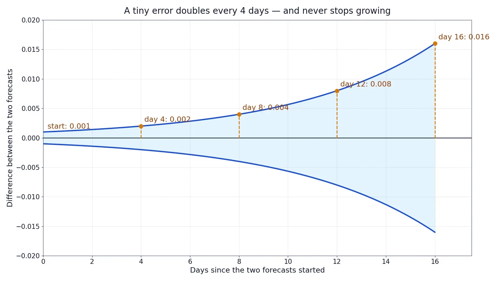
His first thought was that a vacuum tube had failed. That sort of thing happened often enough. But the machine was sound. The difference was in the numbers themselves. The computer held each value to six decimal places. The printout, to save space, showed only three. Lorenz had typed 0.506 where the machine had held 0.506127. The gap was 0.000127, about one part in four thousand — the kind of rounding nobody in 1961 would have thought twice about. And yet that gap, left alone inside a set of equations, grew and grew until it swallowed the whole forecast. Lorenz later described what he found: the differences "more or less steadily doubled in size every four days or so, until all resemblance with the original output disappeared somewhere in the second month."
That coffee break is the best place to begin learning chaos theory, because it contains the whole subject in miniature. The rules were exact. Nothing random was added. No measurement was faked and no equation was wrong. And still the future slipped away — not because the science was sloppy, but because the system itself amplifies small differences until they become large ones. Chaos theory is the study of that amplification. It explains why a butterfly has become the symbol of unpredictability, why weather forecasts hit a wall at about two weeks, why a single short equation can produce behaviour no one can predict by looking at it, and why none of this means the world is random. The world, chaos theory says, is deterministic and unpredictable at the same time. This article works through that apparent contradiction, step by step, with the numbers checked twice.
1. What Is Chaos Theory?
1.1 A working definition
Chaos theory is the study of deterministic systems that are so sensitive to their starting conditions that long-term prediction becomes impossible in practice, even though the rules governing them are exact and contain no randomness at all. A chaotic system is one where two starting points that are almost identical — so close together that no instrument could tell them apart — lead, after enough time, to states that have nothing in common. The technical name for this property is sensitive dependence on initial conditions, and it is the single idea on which the whole subject rests.
Notice what the definition does not say. It does not say the system is random. It does not say the rules are unknown. It does not say the system has no pattern. A chaotic system follows fixed rules, and if you know the starting point exactly and compute with perfect precision, you can predict it forever. The trouble is that "exactly" is not something any real measurement can deliver. Every observation carries a small error, every computer rounds somewhere, and in a chaotic system those small errors do not stay small. They grow, roughly doubling at a steady rate, until they are as large as the thing being predicted. At that point the forecast is worth no more than a guess — not because the physics failed, but because the starting point was never known well enough.
1.2 Three ingredients
Three ingredients have to be present before chaos can appear, and checking for them is the quickest way to tell whether a system is chaotic or merely complicated.
The first ingredient is determinism. The future state of the system must be fixed by its present state through definite rules, with no dice being rolled along the way. The Lorenz equations, which this article works through in section 5, are three ordinary differential equations with no random term anywhere in them. Run them twice from the same starting point and you get the same answer twice. Chaos lives inside determinism; it is not an escape from it.
The second ingredient is nonlinearity. In a linear system, effects add up in proportion to their causes: double the push and you double the result. Most real systems are not like that. In a nonlinear system the output is not proportional to the input, and small causes can have large effects while large causes sometimes have almost none. The logistic map of section 6 is nonlinear because it multiplies the population by one minus the population — that single multiplication is enough to turn a calm, settling system into chaos. Without nonlinearity there is no chaos, which is why the simple linear models of the 1950s could never produce what Lorenz found, however carefully they were built.
The third ingredient is sensitive dependence itself: nearby starting points must separate over time, and the separation must grow roughly exponentially rather than drifting apart slowly. A system where two nearby trajectories separate at a steady walking pace is merely imprecise. A chaotic system is one where the separation multiplies — doubling every few days in Lorenz's weather model, doubling every 0.77 time units in his three-equation system — until the two trajectories are as different as two different systems altogether. The rate of that multiplication has a name, the Lyapunov exponent, and section 4 measures it.
1.3 What chaos theory is not
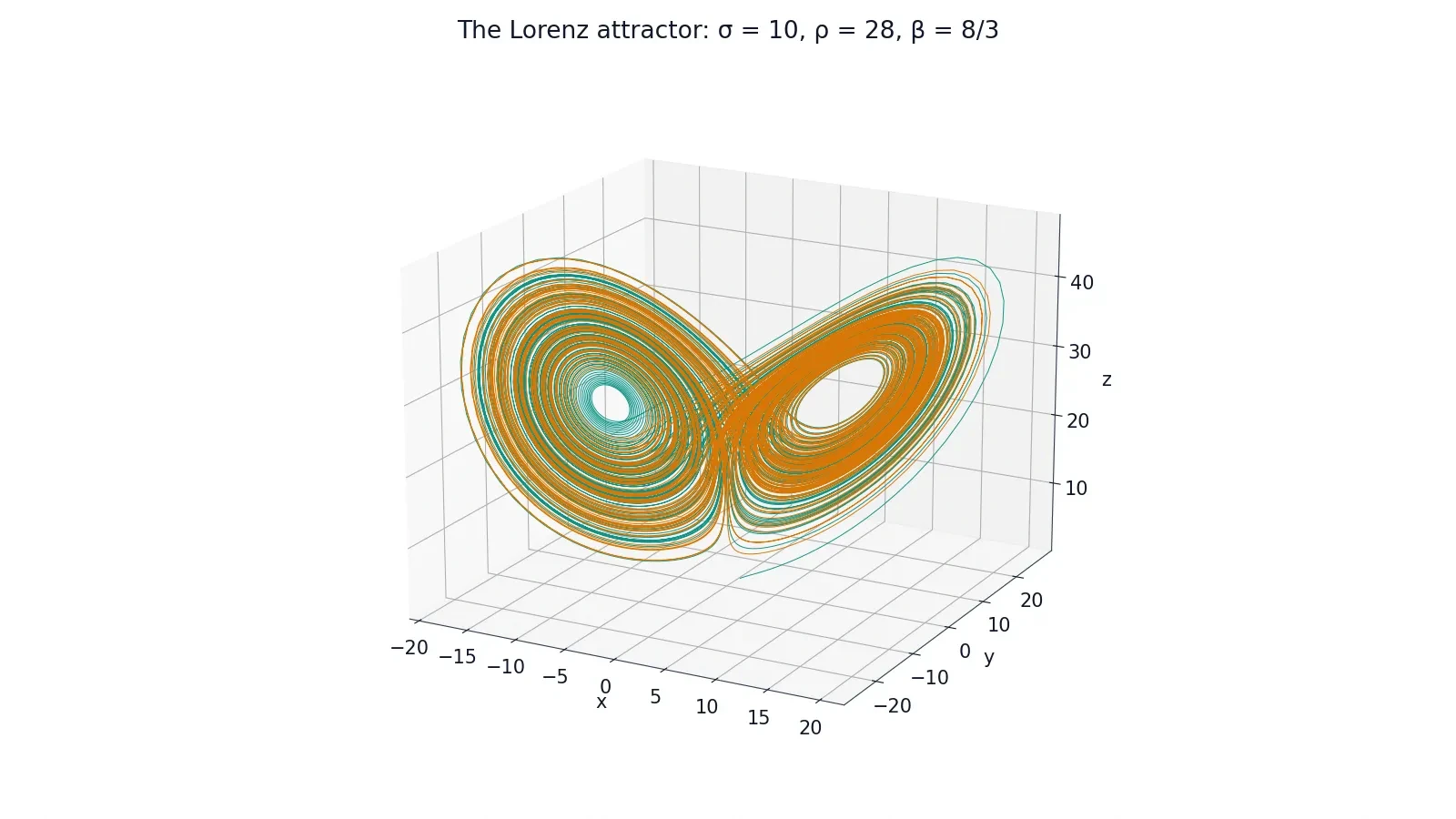
Most people assume chaos means disorder, and that is the first misunderstanding to clear away. A chaotic system is not a mess. The Lorenz attractor, the butterfly-shaped object in the cover image, is a precise geometric structure: every trajectory of the system is drawn toward it, winds around its two lobes, and never leaves it, never repeats itself, and never crosses its own path. That is order of a subtle kind — order in the shape of the motion, even while the timing of the motion defeats prediction. A gas spreading through a room is disordered. A chaotic system is patterned and unpredictable at once, and keeping those two ideas together is the whole skill of the subject.
Chaos theory is also not a theory of everything. It does not say that all systems are chaotic, or that prediction is always hopeless. The motion of the planets over the next century is predictable to high precision. A pendulum swinging through small angles is predictable. Chaos theory draws a line: some systems amplify small errors and some do not, and the interesting question in any given case is which side of the line you are standing on.
I first felt that line under my own hands with a double pendulum — two rods joined end to end, the kind of demonstration that sits on a physics teacher's desk. Release it twice from what looks like the same starting angle, as carefully as you can, and the two swings agree for a few seconds, then disagree, then bear no relation to each other at all. Nothing is wrong with the pendulum. Nothing is wrong with your hands. The system itself takes the tiny difference between your two releases — a difference you cannot see and could not remove — and turns it into a completely different dance. That is chaos theory in a form you can hold, and once you have seen it, the weather forecast starts to make a different kind of sense.
2. The Day the Forecast Broke: Lorenz and the Rounding Error
2.1 The man who found chaos by accident
Edward Norton Lorenz was born on May 23, 1917, in West Hartford, Connecticut, and died on April 16, 2008, in Cambridge, Massachusetts, at the age of 90. He studied mathematics at Dartmouth College, graduating in 1938, and at Harvard, where he took a master's degree in 1940. During the Second World War he served as a weather forecaster for the Army Air Corps, and the experience turned him from pure mathematics toward meteorology. He took his doctorate in meteorology from MIT in 1948 and spent his entire scientific career there, becoming an emeritus professor in 1987.
Lorenz was not looking for a revolution. In the late 1950s he was trying to answer a practical question: could weather be predicted by simulating the physics of the atmosphere on a computer, rather than by the statistical rules of thumb forecasters had always used? He bought one of the first commercial computers available, the Royal McBee LGP-30, an 800-pound machine of vacuum tubes and rotating drum memory that earned its own room on the fifth floor of MIT's Building 24. His programmers were Ellen Fetter and Margaret Hamilton, who later led the software team for the Apollo program. The model Lorenz ran on it had twelve variables — a drastic simplification of the atmosphere, but a real dynamical system with real equations.
2.2 The winter day in 1961
The discovery happened, as the best ones often do, because someone took a shortcut. Lorenz wanted to examine one interesting stretch of a run in more detail. Re-running the whole simulation would have taken hours on his slow machine, so he stopped the computer, typed in a line of numbers from a printout, and set it running again from the middle. Then he went down the hall for a cup of coffee.
When he returned, about an hour later, the machine had simulated roughly two months of weather, and the numbers being printed were nothing like the old ones. He suspected a weak vacuum tube first — a reasonable guess on a machine of that era. But before calling for service he checked where the new run had started to differ from the old one, and what he found changed the direction of his career. The new values at first repeated the old ones, then differed by one unit in the last decimal place, then by several, then in the next-to-last place, then in the place before that. The differences, in his own words, "more or less steadily doubled in size every four days or so, until all resemblance with the original output disappeared somewhere in the second month."
The cause was the rounding. The computer calculated with six decimal places, but the printout showed three, and Lorenz had re-entered the printed numbers as if they were the real ones. Where the machine held 0.506127, he had typed 0.506. The difference was 0.000127 — about 0.025 percent of the value, one part in roughly four thousand. A quick check shows his doubling story holds together: a difference of 0.000127 that doubles every four days needs about 13 doublings to reach a size of 1, and 13 doublings at four days each is 52 days — inside the second month, exactly as he described. Nothing was broken. The equations were simply doing what nonlinear equations do to small differences: amplifying them.
2.3 The 1963 paper
Lorenz distilled the discovery into a paper published in 1963 in the Journal of the Atmospheric Sciences, volume 20, pages 130 to 141, under the modest title "Deterministic Nonperiodic Flow". The title is a thesis in three words: a flow can be deterministic — governed by fixed rules with no randomness — and still never settle into a repeating cycle. In the paper he reduced his twelve-variable model to just three equations describing convection in a layer of fluid heated from below, and showed numerically that essentially all of their solutions are unstable and nonperiodic. Nearby trajectories pull apart exponentially.
The paper's central sentence is worth reading slowly, because it states the whole problem of prediction in one breath:
"It implies that two states differing by imperceptible amounts may eventually evolve into two considerably different states. If, then, there is any error whatever in observing the present state — and in any real system such errors seem inevitable — an acceptable prediction of an instantaneous state in the distant future may well be impossible." — Edward Lorenz, 1963
Lorenz was not saying prediction is useless. He was saying it has a horizon, and that the horizon is set by the system, not by the forecaster.
The paper did not cause a sensation. It was published in a meteorology journal, read mostly by meteorologists, and cited only a handful of times in its first decade outside that field. The idea needed a name, a picture, and a decade of patient work by mathematicians and physicists before it became the subject this article describes. Lorenz himself kept working on it for the rest of his life, collecting the Crafoord Prize in 1983, shared with the oceanographer Henry Stommel, and the Kyoto Prize in 1991. He had finished a paper with a colleague about a week before his death in 2008.
3. The Butterfly Effect: What Lorenz Actually Said
3.1 From seagull to butterfly
The phrase "butterfly effect" did not appear in Lorenz's 1963 paper. It arrived nine years later, and it arrived almost by accident. Lorenz's first version of the metaphor involved a seagull: in a 1963 paper for the New York Academy of Sciences he noted that one meteorologist had remarked that if the theory were correct, one flap of a seagull's wings could change the course of weather forever. The image was vivid but not quite vivid enough, and colleagues kept pressing him for something more poetic.
The chance came in December 1972. Lorenz was to give a talk at the 139th meeting of the American Association for the Advancement of Science, and characteristically he failed to supply a title in time. The session chair, the meteorologist Philip Merilees, supplied one for him: "Predictability: Does the Flap of a Butterfly's Wings in Brazil Set Off a Tornado in Texas?" Lorenz gave the talk on December 29, 1972, and deliberately left the title question unanswered. The phrase escaped the conference hall and never came back.
3.2 The question mark matters
The most common misunderstanding about the butterfly effect is also the most natural one: people hear the phrase and picture a butterfly flapping its wings and somehow powering a tornado thousands of kilometres away, as if the insect were a tiny engine driving the storm. That is not what Lorenz meant, and the question mark at the end of his title is the clue. He was asking a question about predictability, not reporting that a butterfly had been shown to cause a particular tornado.
What the metaphor actually says is this. The flap of a butterfly's wing is a change in the atmosphere so small that it lies below the threshold of any measurement — one thread in a vast web of initial conditions. In a sensitively dependent system, including that thread or leaving it out can, over weeks, place the atmosphere on an entirely different trajectory. The tornado in the title stands for the large-scale state of the system weeks later: whether a storm forms, when it forms, and where it goes. The butterfly does not supply the energy for the storm. A tornado's energy comes from the atmosphere itself, from heat and moisture and wind shear on a scale no insect could touch. The flap is one detail among countless details, and the point is that in a chaotic system no detail is safely negligible.
Lorenz himself was careful about the metaphor in a way his admirers rarely are. He pointed out that "if the flap of a butterfly's wings can be instrumental in generating a tornado, it can equally well be instrumental in preventing a tornado." The small disturbance does not single out catastrophe. It changes the sequence of weather events without necessarily changing how often storms happen over the years. A world with the butterfly is not a world with more tornadoes. It is a world with different tornadoes, on different days, in different places — or with none where one would otherwise have formed.
3.3 The literal reading fails
Taken literally, the butterfly story is false, and working scientists have said so plainly. In a 2024 letter in Physics Today, Roger Pielke, Bo-Wen Shen and Xubin Zeng concluded that a butterfly in Brazil cannot cause a tornado in Texas, because the flap is so small in space and time that molecular dissipation — the atmosphere's own smoothing at tiny scales — wipes it out long before it can grow to weather scales. The butterfly's wing moves air over centimetres; a tornado spans kilometres. Between those scales the atmosphere is full of processes that smear small disturbances away.
That objection does not damage Lorenz's idea. It sharpens it. Lorenz's claim was never about one insect and one storm. It was about the general property of the atmosphere: that errors in our knowledge of its present state, however small, grow until they dominate any forecast. The butterfly is a stand-in for all those errors at once — the temperature between two weather stations, the wind over an empty stretch of ocean, the humidity inside a cloud no instrument has visited. We cannot measure the atmosphere completely, and chaos theory tells us what that incompleteness costs. The metaphor survives because it makes that abstract cost easy to picture, not because entomology causes meteorology.
3.4 Two kinds of butterfly
It helps to separate two claims that the phrase "butterfly effect" is often used to mean. The first claim is the mathematical one: in a chaotic system, a tiny change in the starting conditions can lead to a large change in the later state. That claim is proven, measured, and demonstrated in this article's worked examples. Call it the sensitive-dependence claim, and it is solid.
The second claim is the literal one: that a specific small event, like a butterfly flapping its wings, can organise itself across thousands of kilometres into a specific large event, like a tornado. That claim is a much stronger statement about how small disturbances travel upward through the scales of the atmosphere, and Lorenz himself never verified it. He returned to the question late in life and still treated the answer as open. The honest way to use the phrase is to mean the first claim and to treat the second as a vivid picture of it — a picture, not a report.
4. Sensitive Dependence, Measured
4.1 The Lyapunov exponent
Saying that nearby trajectories "pull apart" is a good start, but science needs a number, and the number has a name: the Lyapunov exponent, named after the Russian mathematician Aleksandr Lyapunov, who studied the stability of motion in the 1890s. The largest Lyapunov exponent, usually written as lambda, measures the average rate at which nearby trajectories separate. If two trajectories start a distance apart that we call epsilon, then after time t their separation is roughly epsilon multiplied by e raised to the power lambda times t. When lambda is negative, trajectories converge and the system is stable. When lambda is zero, they drift apart slowly or not at all. When lambda is positive, they separate exponentially, and the system is chaotic.
For the Lorenz system at its classic parameters, the largest Lyapunov exponent is about 0.906 per unit of time, according to the careful numerical calculation by the physicist Julien Sprott at the University of Wisconsin, who reports the three exponents as 0.9056, 0 and minus 14.5723. The zero in the middle is expected: one exponent of any continuous flow is always zero, corresponding to motion along the trajectory itself. The large negative third exponent tells us the system squeezes volumes in phase space even as it stretches them in one direction — the stretching and squeezing together are what make the attractor. From the largest exponent alone, two useful times follow. The doubling time is the natural logarithm of 2 divided by 0.9056, which is about 0.77 time units: that is how long it takes any small error to double. The e-folding time, the time for an error to grow by a factor of e, is 1 divided by 0.9056, about 1.10 time units.
4.2 A worked example: two Lorenz runs
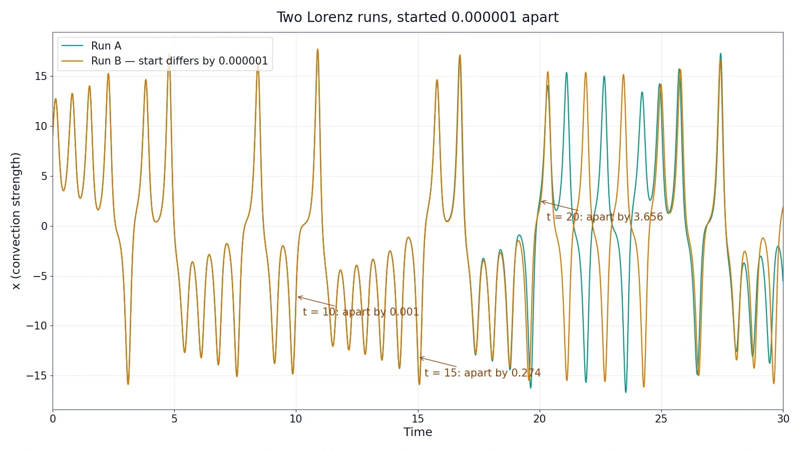
Numbers like these are more convincing when you watch them happen, so I integrated the Lorenz equations twice, with a fourth-order Runge–Kutta integration with a step of 0.01 time units, starting from a point already on the attractor: (8.813271, 12.901260, 20.914967), reached by integrating 5,000 steps from (1, 1, 1). The exact starting point matters — even the rounded coordinates found in most retellings give a different table, which is itself a small demonstration of the effect. The two runs were identical except for one detail — the starting x value of the second run was larger by 0.000001, one part in a million. Everything else, the equations, the parameters, the other two starting values, was the same.
The table below shows the distance between the two trajectories as time passes. The growth is not smooth, and that unevenness is itself part of the lesson: chaos amplifies errors in bursts, when the trajectory swings past an unstable region, and lets them shrink briefly at other times. But the direction of travel is unmistakable.
Time | Separation between the two runs | What the runs look like |
|---|---|---|
0 | 0.000001 | Identical to six decimal places |
5 | 0.000032 | Still identical to the eye |
10 | 0.000728 | A difference in the third decimal place |
15 | 0.274032 | Clearly different trajectories |
20 | 3.656403 | On different parts of the attractor |
25 | 7.598502 | Often on opposite wings |
30 | 14.890186 | No resemblance left |
A one-in-a-million difference in the starting point became a difference of about 15 — as large as the attractor itself — in 30 time units. The arithmetic of the exponent predicts the same story in a smoother form: an error of one millionth, growing by a factor of e every 1.10 time units, needs the natural logarithm of one million, about 13.82, e-foldings to reach a size of 1, and 13.82 times 1.10 is about 15.3 time units. The measured table and the exponent agree. By 15 time units the separation is already 0.27 and climbing fast.
4.3 Why this defeats prediction
The worked example explains why better measurements alone cannot save long-term forecasting. Suppose you could measure the starting state of the atmosphere ten times more precisely than today. In a system with a doubling time of a few days, that improvement buys you only about three more doublings of lead time — roughly ten to fifteen extra days of forecast, not a lifetime of it. Every factor-of-ten improvement in measurement buys a fixed, modest extension of the horizon, because the error grows exponentially while your improvement is only multiplicative. To forecast twice as far ahead, you would need to measure the starting state exponentially more precisely, and there is a floor set by physics itself: below a certain scale, the atmosphere is made of molecules, and no measurement can be more precise than the molecular grain.
This is also why chaos theory is not an argument against forecasting. Short-term forecasting works, and it works well, precisely because the errors have not yet had time to grow. A one-day forecast is excellent; a five-day forecast is good; a ten-day forecast is a guide to trends. The horizon is not a wall that appears suddenly. It is a slope, and chaos theory measures the slope.
5. The Lorenz Attractor: Three Equations, One Butterfly
5.1 Three equations from a pot of soup
Lorenz's great simplification was to take the physics of convection — a layer of fluid heated from below, like soup in a pot — and keep only the three features that matter most. Warm fluid rises, cool fluid sinks, and the rising and falling organise into rolls. Lorenz represented the strength of the convection roll by x, the temperature difference between rising and falling fluid by y, and the departure of the vertical temperature profile from a straight line by z. Three numbers, changing in time, stand in for the whole weather system.
The equations are short enough to write on a postcard:
dx/dt = σ(y − x)
dy/dt = x(ρ − z) − y
dz/dt = xy − βz
The first equation says the convection strength chases the temperature difference. The second says the temperature difference is driven by the convection and damped by its own size. The third says the temperature profile is bent by the product of the convection and the temperature difference, and relaxes back at a rate set by β. The only nonlinearity in the whole system is the multiplication of two variables: x times z in the second equation, x times y in the third. Two multiplications are all it takes.
5.2 What the parameters mean
The three parameters are not arbitrary knobs. Each one stands for a physical property of the fluid. Sigma, σ, is the Prandtl number, the ratio of how quickly momentum spreads through the fluid to how quickly heat spreads through it. For air σ is about 0.72; Lorenz used σ = 10, which suits water better but gives robust chaos, and the choice has become the standard. Rho, ρ, is the Rayleigh number relative to its critical value — a measure of how hard the fluid is being driven by the heating from below. Beta, β, is a geometric factor related to the shape of the convection cell, and the classic value is 8/3, about 2.667.
Lorenz used the values σ = 10, ρ = 28 and β = 8/3, and they have become the classic parameters of chaos theory, the ones every textbook and simulation uses. At these values the system is chaotic. But the chaos is not present for every choice of ρ. Turn the heating down and the system settles: for low ρ the fluid sits still, and for middling ρ it settles into steady convection rolls. The chaos switches on only past a threshold, and the threshold can be calculated exactly.
5.3 Fixed points, and why none of them holds
A fixed point is a state where all three rates of change are zero — a place where the system, if put there exactly, would stay forever. The Lorenz system has three of them. One is the origin, (0, 0, 0), the state of no motion at all. The other two are mirror images, C+ and C−, sitting at the centres of the two lobes of the butterfly. Their coordinates are plus and minus the square root of β times (ρ − 1) for x and y, and ρ − 1 for z. With the classic parameters that is the square root of 8/3 times 27, which is the square root of 72, about 8.485, for x and y, and 27 for z. So C+ is at (8.485, 8.485, 27) and C− at (−8.485, −8.485, 27).
The important fact about these fixed points is that at ρ = 28 none of them is stable. The origin loses its stability early, and the two lobe centres lose theirs at a Hopf bifurcation when ρ reaches about 24.74 — the value of σ times (σ + β + 3) divided by (σ − β − 1), which works out to 10 times 15.667 divided by 6.333, or 24.74. Past that value, a trajectory that spirals toward one of the lobe centres is pushed away from it instead, spirals outward, and is flung across to the other lobe, where the same thing happens again. It never settles, never repeats, and never escapes. That endless switching between two unstable centres is the motion you see in the butterfly.
5.4 The strange attractor
The set of points the trajectory visits, the butterfly itself, is called the Lorenz attractor, and it is a strange attractor. "Attractor" because trajectories from a wide range of starting points are drawn toward it and stay on it. "Strange" because its geometry is fractal: it has structure on every scale, and its dimension is not a whole number.
The dimension can be computed from the Lyapunov exponents by the Kaplan–Yorke formula: take 2, and add the largest exponent divided by the size of the most negative one. That is 2 plus 0.9056 divided by 14.5723, which is 2.06215. The attractor is therefore about 2.06-dimensional — more than a surface, which would be 2, and far less than a solid, which would be 3. The correlation dimension, measured differently, comes out at about 2.05, confirming the same picture. What this means in plain language is that the trajectory winds around an object that is infinitely folded: it has the area of a surface but is crumpled so finely that it almost fills a volume, without ever quite doing so. If you zoom into any part of it, you find the same layered structure again, like the coastline of a fractal island.
The attractor also explains why the butterfly shape became the symbol of the field. Plot the trajectory in three dimensions and you get two lobes that look, from the right angle, like a pair of wings. The resemblance is a coincidence of the viewing angle — the attractor is not really a butterfly, and the butterfly in the metaphor is not really the attractor — but the image stuck because it is beautiful, and because it makes an abstract object visible. Every point on those wings is a possible state of the system, and the trajectory wanders over them forever, never visiting the same point twice, never leaving the wings.
5.5 Deterministic, but never repeating
The strangest property of the attractor is the combination it embodies. The motion is fully deterministic: the equations fix the future exactly. The motion is bounded: it never leaves the wings. And yet it is nonperiodic: it never repeats a state, never closes into a loop, never settles into a cycle. Many textbooks still assumed that a deterministic system with bounded motion must eventually repeat itself or settle down — Poincaré's 1890 exception had been largely forgotten. Lorenz showed that assumption is false. A deterministic system can wander forever inside a bounded region without ever repeating, and that wandering is what makes long-term prediction impossible while short-term prediction remains perfectly sensible.
6. The Logistic Map: Chaos from One Line
6.1 One equation, a whole zoo
If the Lorenz system is chaos with three equations, the logistic map is chaos with one line, and it is the clearest demonstration that complexity does not need complicated rules. The map describes a population that grows and then is held back by limited resources. Let x be the population as a fraction of the maximum the environment can support, so x always lies between 0 and 1, and let r be the growth rate. Then the population in the next generation is:
x next = r times x times (1 − x)
The term (1 − x) is the brake: when the population is small, the brake is barely applied and the population grows; when the population is close to the maximum, the brake bites hard and the population falls. The equation comes from the logistic curve of the Belgian mathematician Pierre-François Verhulst, published in 1838, and it was the biologist Robert May who showed what it could do. In his 1976 paper in Nature, "Simple mathematical models with very complicated dynamics", May took this one line and showed that it contains fixed points, oscillations, period doubling, and full chaos — a whole zoo of behaviour hiding inside a single multiplication.
6.2 Worked example: settling down
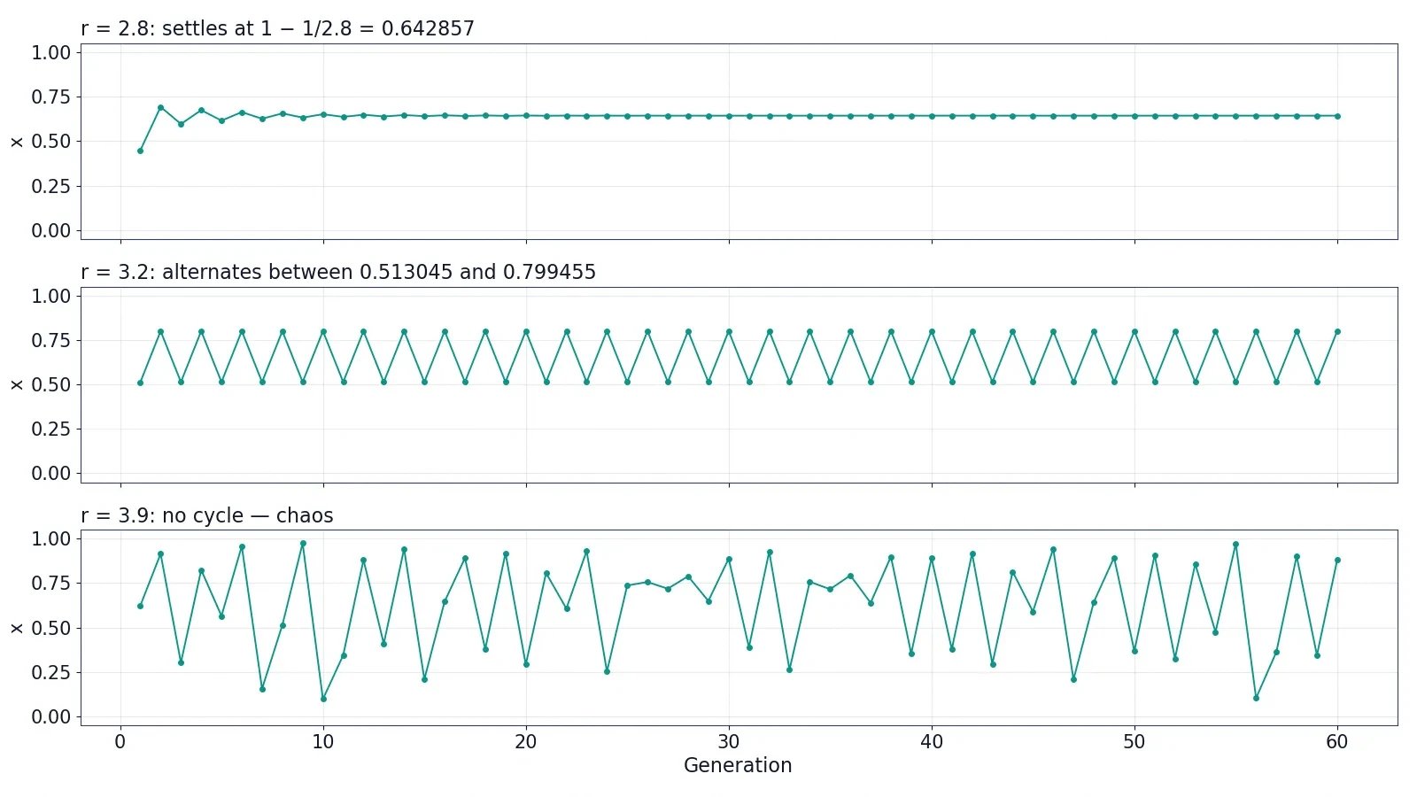
Start with r = 2.8 and an initial population of 0.2, one fifth of the maximum. The rule is easy to apply by hand, so follow the arithmetic. The fixed point of the map, the value where the population stays the same from one generation to the next, is 1 minus 1 divided by r. For r = 2.8 that is 1 minus 0.357143, which is 0.642857. Iterate the map and the population climbs toward that value and stays there: 0.2, then 0.448, then 0.692, then 0.596, then 0.674, and after a few dozen generations it is sitting at 0.642857, generation after generation. The system has a stable fixed point. Measure the starting population a little differently and the same value results. This is the calm regime, and it is how most people expect mathematics to behave.
6.3 Worked example: the two-cycle
Now raise the growth rate to r = 3.2 and start again from 0.2. The fixed point is now 1 minus 1 divided by 3.2, which is 0.6875 — but the population no longer settles there, because at r = 3.2 the fixed point has become unstable. Watch the iterates, computed step by step. The first is 3.2 times 0.2 times 0.8, which is 0.512000. The second is 3.2 times 0.512 times 0.488, which is 0.799539. The third is 3.2 times 0.799539 times 0.200461, which is 0.512884. The fourth is 0.799469. The values are closing in on two numbers, not one: 0.513045 and 0.799455. From then on the population alternates between them, high one generation, low the next, forever. The system has undergone its first period doubling: a stable fixed point has given way to a stable two-cycle. Start from any other initial value and you end up on the same two-cycle. The behaviour is still perfectly predictable — you just need to know which of the two values comes next.
I first worked this calculation out on paper, late one evening, expecting the numbers to settle and being quietly startled when they did not. There is something unnerving about a rule this short refusing to sit still, and that unnerving feeling is the honest response. The equation is not misbehaving. It is showing you the first step on the road to chaos.
6.4 Worked example: chaos itself
Raise the growth rate to r = 3.9 and the picture falls apart. There is no cycle to settle into, short or long. The population jumps from value to value with no visible pattern, and — here is the decisive test — two populations that start almost identically now diverge exactly the way Lorenz's weather model did. Take x0 = 0.200000 and x0 = 0.200001, a difference of one part in a million, and iterate both with r = 3.9. After 1 step the difference is 0.000002. After 5 steps it is 0.000028. After 10 steps it is 0.000057. After 13 steps it is 0.000641. After 15 steps it is 0.001563. After 18 steps it is 0.012298. After 20 steps it is 0.039082. After 22 steps it is 0.150037. After 25 steps it is 0.320212. And after 30 steps the two populations are 0.887619 and 0.253293 — a difference of 0.634327, more than half the entire range of the system, from starting points that differed by one millionth. The numbers are not random: each one follows exactly from the one before by a rule a child could apply. But knowing the rule does not help you predict the 30th value from the first one unless you know the first one to more than six decimal places, and no measurement of a real population is that precise.
For completeness, here is the extreme case, r = 4.0, starting from 0.2: 0.640000, 0.921600, 0.289014, 0.821939, 0.585421, 0.970813, 0.113339, 0.401974, 0.961563, 0.147837. Ten values, no pattern a reader could use to guess the eleventh, every one of them produced by the same one-line rule. At r = 4.0 the map is fully chaotic, and it is also a precise mathematical fact that its behaviour is equivalent to a coin toss written in binary — a connection this article's companion piece on what is probability explores from the other side, through the mathematics of chance itself.
6.5 Why one line is enough
The logistic map matters because it removes every excuse. The Lorenz system has three equations and a computer behind it; a sceptic could wonder whether the chaos came from the complexity of the machinery. The logistic map has one equation, one multiplication, and nothing else — and it still produces chaos. That tells us chaos is not a property of complicated systems. It is a property of nonlinear rules, and nonlinear rules are everywhere. May's paper was about insect populations, but the same mathematics turns up in economics, in electronics, in chemistry, and in the beating of the heart. The simplicity is the point: if a single line can do this, then any system with a similar nonlinearity in it can do it too.
7. Period Doubling and the Feigenbaum Constant
7.1 The cascade
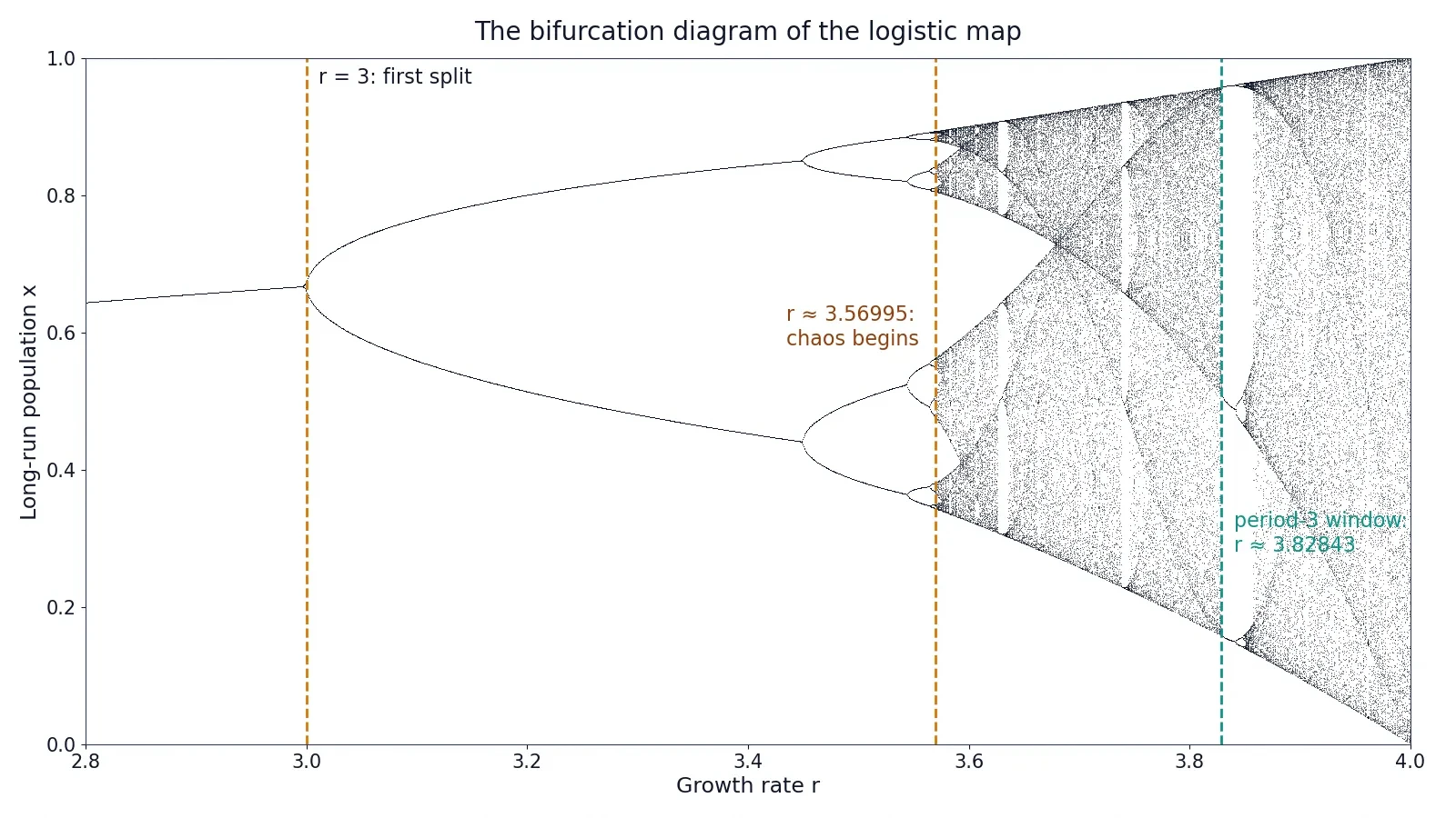
The logistic map does not jump from calm to chaos in one step. It gets there by doubling, again and again, in a pattern so regular that it has its own universal number. At r below 3, the map settles to a single value. At r = 3 exactly, that fixed point loses its stability and a two-cycle is born. Raise r further and the two-cycle loses its stability in turn, giving way to a four-cycle. Then an eight-cycle, a sixteen-cycle, a thirty-two-cycle — each doubling arriving faster than the one before, the intervals between doublings shrinking by a nearly constant factor, until the doublings pile up at a finite limit and the period becomes effectively infinite. That limit is the onset of chaos.
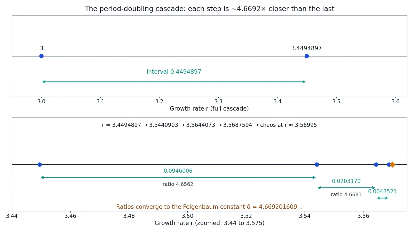
The bifurcation points — the exact values of r where each doubling happens — are known precisely. The first is r = 3. The second is r = 3.4494897. The third is r = 3.5440903. The fourth is r = 3.5644073. The fifth is r = 3.5687594. The cascade accumulates at r ≈ 3.56995, beyond which the behaviour is, from almost all starting points, chaotic. Between the doublings the system is perfectly periodic and predictable; past the accumulation point it is not. The road to chaos is therefore not a cliff but a staircase with steps that shrink geometrically, and the shrinking has a fixed ratio.
7.2 A universal number
Take the intervals between successive bifurcation points and divide each one by the next. The first interval is 3.4494897 minus 3, which is 0.4494897. The second is 3.5440903 minus 3.4494897, which is 0.0946006. The third is 0.0203170. The fourth is 0.0043521. Now the ratios: 0.4494897 divided by 0.0946006 is 4.7514. Then 0.0946006 divided by 0.0203170 is 4.6562. Then 0.0203170 divided by 0.0043521 is 4.6683. The ratios are converging, and their limit is a number called the Feigenbaum constant, delta, equal to 4.669201609…
The physicist Mitchell Feigenbaum discovered this number in 1975, working with a hand calculator at Los Alamos, and published the analysis in 1978 and 1979 in the Journal of Statistical Physics. What makes the number extraordinary is not its value but its reach. The same constant, 4.669201609…, turns up in completely different systems that follow the same route to chaos: in fluid convection experiments, in electronic circuits, in lasers, in chemical reactions. It does not depend on the details of the system. Any one-dimensional map with a single smooth hump — the logistic map, the sine map, and many others — produces the same ratio. It is a universal number in the same sense that pi is universal: it belongs to the mathematics, not to the particular physical system, and it shows up wherever the same mathematics applies.
There is a second Feigenbaum constant, alpha, equal to about 2.5029, which governs how the shape of the map rescales at each doubling. The two constants together were explained in the 1980s by renormalisation theory, the same circle of ideas that explains universality in phase transitions, and the conjectures were eventually proved with computer-assisted methods and then by a full mathematical proof. The logistic map, a single line of arithmetic, turned out to be a window onto one of the deepest structures in mathematics.
7.3 Islands of order inside chaos
Past the accumulation point, the diagram is not featureless noise. Bright vertical stripes cut through the chaotic bands — windows where the system suddenly becomes periodic again. The widest and most famous is the period-3 window, centred at r = 1 plus the square root of 8, which is 3.828427…, where the map settles into a three-cycle, visiting values close to 0.160, 0.514 and 0.956 in rotation. Inside that window the period doubles again — three becomes six, six becomes twelve — and chaos returns, in miniature, through the same cascade.
The period-3 window matters for a theorem as well as for the picture. In 1975 the mathematicians Tien-Yien Li and James Yorke proved that any continuous map of an interval that has a point of period three must also have points of every other period, and must be chaotic. Their paper, "Period three implies chaos", gave the field one of its most quoted slogans, and it also gave chaos its name in the mathematical literature: the word "chaos" in its technical sense comes from that paper. The window in the diagram is the visible trace of the theorem.
8. Chaos Is Not Randomness
8.1 The distinction that matters most
If this article has a spine, it is the distinction between chaos and randomness, and it is worth stating as plainly as possible. Chaos is deterministic. Randomness is not. A chaotic system follows fixed rules with no element of chance, and if you know its exact starting state you can predict its exact future. A random process, like a coin toss or radioactive decay, has no exact future to know: the same starting conditions can lead to different outcomes, and no amount of information about the present will tell you which one will happen. Chaos is a limit on prediction in practice. Randomness is a limit on prediction in principle. They are different limits, and confusing them is the most common error people make about this subject.
The confusion is understandable because chaotic and random behaviour look alike from the outside. The logistic map at r = 4.0 produces a sequence of numbers that passes many statistical tests for randomness. The Lorenz trajectory looks irregular. But the resemblance is only skin deep, and there are tests that separate them cleanly. A chaotic system has a strange attractor — a geometric structure that its trajectories never leave. A random process has no attractor. A chaotic system has a positive Lyapunov exponent but a bounded state space. A random walk wanders without bound. A chaotic system is predictable in the short term and unpredictable in the long term. A random process is unpredictable at every timescale, including the next step.
8.2 A comparison
Property | Chaotic system (Lorenz, logistic map) | Random process (coin toss, dice) |
|---|---|---|
Rules | Fixed and exact, no chance involved | Outcomes governed by probability |
Same start, same result? | Yes, always | No, outcomes vary |
Short-term prediction | Accurate while errors stay small | Impossible beyond the odds |
Long-term prediction | Defeated by error growth | Defeated by chance itself |
Underlying structure | Strange attractor with fractal dimension | No attractor, no structure to find |
What more data buys | A modestly longer forecast horizon | Nothing about the next outcome |
The last row is the practical test. Give a forecaster ten times better measurements of a chaotic system and the forecast horizon extends by a few doubling times. Give a gambler ten times more data about a fair coin and the next toss is still a coin toss. Chaos rewards better information, just not enough of it. Randomness does not reward it at all.
8.3 Why the confusion persists
The confusion persists for a respectable reason: in real life, the two are often mixed together. The weather is chaotic and also noisy — measurement errors, unresolved small-scale processes, and genuine randomness at the molecular level all feed into the same forecast. A heart rhythm is chaotic and also influenced by breathing, posture, and hormones. A stock price is influenced by chaotic dynamics and by genuinely unpredictable news. Separating the chaotic part from the random part is a real scientific problem, and researchers do it with tools like Lyapunov exponents and attractor reconstruction, which test whether a time series has the geometric signature of chaos or the flat signature of noise.
There is also a philosophical edge to the distinction, and it is worth one paragraph. Before Lorenz, the prevailing view — associated with the French mathematician Pierre-Simon Laplace — was that a sufficiently powerful intelligence, knowing the exact state of the world, could predict its entire future. Lorenz showed that even with perfect laws, prediction fails in practice because the exact state can never be known. But notice what he did not show: he did not show that the future is open, or that chance rules the world, or that determinism is false. The future of a chaotic system is fixed by its present state. It is simply unknowable to us beyond a horizon, because knowing the present state exactly would require infinite precision. Determinism survives. What dies is the hope of using determinism to predict everything. Lorenz put the point in a single sentence: when the present determines the future, but the approximate present does not approximately determine the future.
This is where the mathematics of probability, covered in this site's what is probability article and in the companion piece on how statistics can mislead, meets chaos theory from the other side. Probability describes systems where the future genuinely branches. Chaos theory describes systems where the future is single but hidden behind a wall of amplification. Both are needed to understand why prediction is hard, and neither alone is enough.
9. Why We Cannot Predict the Weather
9.1 The two-week wall
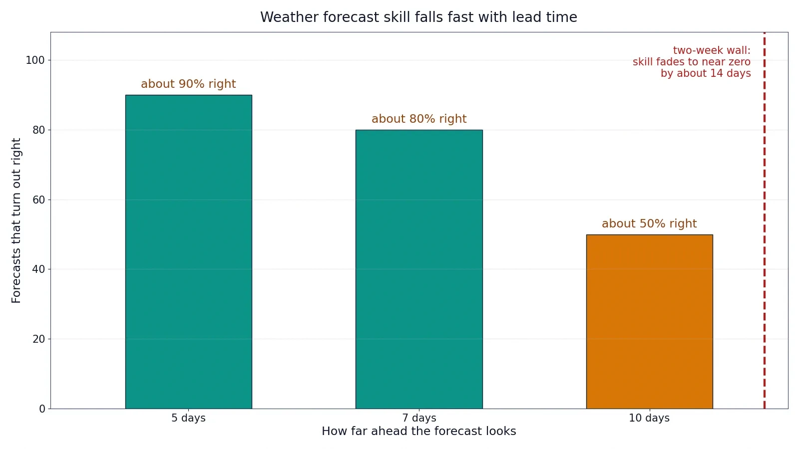
The most famous consequence of chaos theory is also the most familiar: you cannot know next month's weather in detail, no matter how good the computers get. The limit is usually quoted as about two weeks, and its history is worth knowing because the number does not come from Lorenz alone. Lorenz's 1969 paper, "The predictability of a flow which possesses many scales of motion", framed the problem, but the two-week figure itself traces back to a 1966 study by Jule Charney and colleagues, who found that errors in a first-generation general circulation model doubled in about five days. Extrapolate that growth — an error doubling every five days grows by a factor of about 7 in fourteen days — and the forecast has lost its skill by the end of the second week. Lorenz himself later acknowledged that his 1969 model was too simple to settle the atmosphere's true limit, because it left out processes like baroclinic instability and dissipation that shape real error growth. The two-week figure has survived half a century of better models and faster computers because the underlying reason for it — exponential error growth in a chaotic atmosphere — has survived too.
The ladder of forecast accuracy shows the slope clearly. NOAA's widely quoted figures put a five-day forecast right about 90 percent of the time and a seven-day forecast at about 80 percent, while a ten-day forecast is accurate only around half the time. By day fourteen the forecast is near the practical limit: a rough signal of trends, not a reliable day-by-day plan. The modern five-day forecast is about as accurate as a one-day forecast was several decades ago — a genuine triumph of satellites, computing, and better physics — and yet the horizon has barely moved. The improvement went into accuracy within the horizon, not into extending the horizon itself. That is exactly what chaos theory predicts: better measurements and better models push the error down, but the exponential growth eats the improvement in a fixed number of doublings.
9.2 Ensembles: forecasting with many worlds
The practical answer to chaos in weather forecasting is the ensemble. Instead of running one forecast from one best guess at the present state, centres like the European Centre for Medium-Range Weather Forecasts and the US National Weather Service run the model many times — dozens of times — from slightly different starting conditions and with slightly different physics. Each run is a possible world. Where the runs agree, the forecast is confident. Where they spread apart, the forecast is uncertain, and the spread itself is the honest measure of that uncertainty.
Ensembles work because they turn the weakness of chaos into information. A single run pretends to know the future; an ensemble admits that it does not, and shows you the range of futures consistent with what is known. The European centre's high-resolution forecast runs to 15 days, and the American GFS model to 16 days, but the useful skill — the range where the forecast beats simply guessing the average weather for the date — fades well before that. Modern research has refined the limit rather than removed it: a 2019 study by Fuqing Zhang and colleagues found that cutting today's initial-condition error by a factor of ten would extend midlatitude skill to about 15 days, and ensemble studies put marginal skill at up to about 23 days. These are refinements of the same wall, not holes in it.
I learned to read ensemble forecasts the practical way, planning a trip around a forecast ten days out and watching it change every day. On the first day the forecast promised sun. Three days later it promised rain. By the day itself it was cloudy with a shower in the afternoon, and none of the earlier versions had been wrong in the way a liar is wrong. Each had been the best estimate from the information available at the time, and the information changed as the atmosphere moved. The forecast was not failing. It was doing exactly what a chaotic system allows a forecast to do: be right for a while, then diverge.
9.3 Weather is not climate
One more distinction matters, because it is where public discussion of this subject most often goes wrong. The two-week limit applies to weather — the day-to-day state of the atmosphere. It does not apply to climate, which is the long-term average of weather over seasons, years, and decades. Climate prediction is a different problem, not a longer weather forecast. It asks how the statistics of weather change when the boundary conditions change — when greenhouse gases rise, when the oceans warm, when the ice retreats. Those boundary conditions are predictable in a way that tomorrow's rain is not, and the equations that describe the energy balance of the planet are not the same as the equations that describe a particular storm. Chaos limits the first kind of prediction. It does not forbid the second.
The machinery of weather forecasting — numerical weather prediction, satellites, data assimilation, ensembles — is a subject in its own right, and this site's Meteorology Explained article covers it in full, from how the models are built to how a forecast is made. This article has used only the one fact from that story that belongs to chaos theory: that the atmosphere is a chaotic system, and that this sets a horizon no model can cross by much.
10. Chaos in the Real World
10.1 Poincaré and the three-body problem
Chaos was discovered before Lorenz, and its first discoverer did not know what he had found until a mistake forced him to look. In 1885, King Oscar II of Sweden offered a prize for solving the n-body problem of celestial mechanics: given the positions and velocities of three or more bodies pulling on each other by gravity, predict their motion. The French mathematician Henri Poincaré entered, and on January 21, 1889, he won. His memoir was being typeset for publication when he found a serious error in his proof — he had claimed a stability that was not there. Phragmén's editorial queries led Poincaré himself to find the error, and Poincaré paid out of his own pocket to recall and reprint the published copies, a sum reported to exceed the prize itself.
Repairing the error led him to something far more important than the prize. Poincaré discovered that the stable and unstable trajectories of certain orbits do not simply miss each other or join smoothly, but intersect infinitely often, weaving a structure of unimaginable complexity that he called a homoclinic tangle. In his later book Les méthodes nouvelles de la mécanique céleste he wrote that he would not even attempt to draw it. That tangle is the mechanism of chaos: nearby trajectories separate exponentially, and long-term prediction of the three-body system becomes impossible in principle. His corrected memoir, published in 1890 in Acta Mathematica, is the foundation of dynamical systems theory — chaos theory discovered seventy years before the word, by a man trying to fix a mistake. Two bodies orbiting each other trace perfect ellipses, solved by Newton. Add a third body and the formula vanishes. The solar system is stable over human timescales, but its inner planets have a Lyapunov time — the time for small differences to grow by a factor of e — of only about five million years, short compared with the age of the solar system itself.
10.2 The double pendulum and the dripping tap
Chaos is not confined to the sky and the weather. It sits on tabletops. A double pendulum — one pendulum hanging from the end of another — is deterministic, simple to build, and chaotic for most starting angles. Give it a push, watch it swing, and the motion is graceful for a few seconds and then wild, flipping and tumbling in a way no eye can follow. Start it twice from the same position and the two motions agree briefly and then part company, exactly as Lorenz's trajectories did. It is the same phenomenon at human scale, and it is why the double pendulum has become the standard classroom demonstration of chaos.
A dripping tap does the same thing with water. As the flow rate increases, the drips go from a steady rhythm to a doubled rhythm — two different intervals alternating — to a quadrupled rhythm, and then to irregular dripping with no pattern at all. Robert Shaw proposed the dripping faucet as a model chaotic system in 1984, and the experiment has been repeated many times since: the route to chaos is the same period-doubling cascade as the logistic map, with the same Feigenbaum constant waiting at the end of it. I have stood at a kitchen sink and watched a tap do this, turning the handle a fraction at a time, and the ordinariness of it is the point. Chaos does not need exotic equipment. It needs a nonlinearity and a little patience.
10.3 The beating heart
The most consequential place chaos turns up is inside the body. A healthy heartbeat is not a metronome. The interval between beats varies from moment to moment in a complex, irregular pattern, and that irregularity is not noise — it has fractal structure, the same kind of self-similarity at different scales that the Lorenz attractor shows. The cardiologist Ary Goldberger and his colleagues showed, in work published in Scientific American in 1990 and developed since, that the healthy heart displays the hallmarks of a nonlinear dynamical system, and that disease often shows up as a loss of that complexity: the heartbeat becomes too regular, too periodic, as the system loses its healthy variability. Goldberger's PhysioNet tutorial on nonlinear dynamics for clinicians works through the same ideas with real heart-rate records. A heart that beats with perfect regularity is not a healthy heart. It is a heart whose control systems have lost their flexibility.
The same mathematics appears in the electrical activity of the heart, where period-doubling cascades in cardiac action potentials can precede chaotic early afterdepolarisations — irregular voltage oscillations that are potential precursors of arrhythmias. Chaos theory in medicine is not a metaphor. It is a diagnostic lens, and it is one more reason the subject matters beyond the blackboard.
10.4 Populations, circuits, and lasers
Robert May's logistic map began as a model of insect populations, and population dynamics remains one of the clearest applications: a species with a high growth rate and limited resources can fluctuate chaotically from year to year, so that two nearly identical starting populations end up on completely different trajectories — a warning against confident long-term predictions in ecology and fisheries. The same period-doubling route, with the same Feigenbaum constant, has been measured in fluid convection, in electronic circuits, and in lasers, confirming that universality is not a mathematical curiosity but a fact about the physical world. Wherever a system is driven harder and harder through a sequence of doublings, the number 4.669201609… is waiting.
11. Fractals: The Geometry of Chaos
11.1 The shape of a chaotic system
Chaotic motion needs a place to live, and that place turns out to have a strange geometry. A trajectory that never repeats itself, inside a bounded region, must fold back on itself forever without ever crossing its own path — and the only way to do that is to be infinitely layered. The result is a fractal: a shape with detail at every scale, so that zooming in reveals the same kind of structure again and again. The Lorenz attractor is one. The bifurcation diagram is another: zoom into the period-3 window and you find a smaller copy of the whole diagram inside it, cascade and all.
The word "fractal" was coined by the mathematician Benoit Mandelbrot in 1975, and his book The Fractal Geometry of Nature, published in 1982, showed that such shapes are everywhere in the natural world: in coastlines, in clouds, in mountain ranges, in the branching of blood vessels and trees. Mandelbrot's insight and Lorenz's discovery are two sides of the same coin. Chaos is what happens in time when a system is sensitively dependent. Fractals are what the system looks like in space when you draw its behaviour. The attractor is the fractal; the motion on it is the chaos.
11.2 The snowflake that never ends
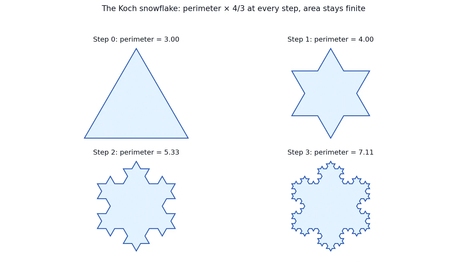
The cleanest fractal to build by hand is the Koch snowflake, invented by the Swedish mathematician Helge von Koch in 1904. Start with an equilateral triangle. Take each straight edge, divide it into three equal parts, and replace the middle third with two sides of a smaller triangle sticking outward. Repeat. Each step replaces every segment with four segments, each one third as long, so the perimeter multiplies by 4/3 at every step. After one step a triangle of perimeter 3 has perimeter 4. After five steps it is 3 times (4/3) to the power 5, which is 12.64. After ten steps it is 53.27. The perimeter grows without bound — after enough steps it exceeds any length you care to name — while the area enclosed stays finite, converging to a fixed value only about 1.6 times the area of the original triangle. An infinitely long boundary around a finite area: that is what fractal geometry means, and it is the same paradox the Lorenz attractor embodies, a trajectory of infinite length folded into a finite region.
11.3 Between dimensions
The Koch snowflake has a dimension between 1 and 2: it is more than a line and less than a surface, just as the Lorenz attractor, at dimension 2.06, is more than a surface and less than a solid. Ordinary geometry has no room for such numbers, and for centuries they were treated as curiosities. Chaos theory made them central, because the dimension of an attractor measures how much room the system's behaviour needs. A periodic system lives on a loop, dimension 1. A quasiperiodic system lives on a torus, dimension 2. A chaotic system needs a fractional dimension, because its behaviour is richer than any smooth surface can hold and poorer than a solid volume. Measuring the dimension of a time series — from a heartbeat, from a dripping tap, from a weather record — is now a standard way to test whether chaos is present.
Fractals deserve a full article of their own, and this cluster has one planned: Fractals Explained is Mathematics article 17, where the Mandelbrot set, the Koch snowflake, and fractals in nature get the deep treatment. Here they appear only as the geometry of chaos, because that is the role they play in this story: the shape that sensitive dependence draws in space.
12. Common Mistakes About Chaos
12.1 Six misunderstandings, corrected
Chaos theory is one of the most misquoted subjects in science, and the mistakes follow a pattern. Each of the six below is something I have heard from intelligent people, and each has a short correction.
A butterfly causes a tornado. No. A butterfly's flap is one detail among countless details in the atmosphere's starting state, and it supplies no energy to any storm. In a chaotic system the flap can change which weather happens weeks later — or prevent a storm as easily as generate one, as Lorenz himself stressed. The literal claim that one insect causes one tornado is false, and working atmospheric scientists have said so in print.
Chaos means randomness. No. Chaos is deterministic: same start, same result, every time. Randomness means the future genuinely branches. The logistic map at r = 4.0 looks random and is not. The difference matters because it decides what better information can buy you: in a chaotic system it buys a longer forecast; in a random system it buys nothing about the next outcome.
Chaos means no patterns. No. Chaotic systems have some of the most beautiful patterns in mathematics — the Lorenz attractor, the bifurcation diagram, the fractal structure of a heartbeat. The pattern is in the shape of the motion, not in the timing of it. A system can be perfectly patterned and still unpredictable in detail.
More computing power will fix forecasting. Not by much. A tenfold improvement in measurement buys only a few extra days of forecast, because errors grow exponentially. Faster computers have made forecasts far more accurate within the two-week horizon, and they will keep doing so, but the horizon itself moves only slowly. It is set by the atmosphere, not by the hardware.
Chaos means anything can happen. No. A chaotic system is confined to its attractor. The Lorenz trajectory never leaves its two wings, the logistic map never leaves the interval from 0 to 1, and a dripping tap never drips upward. Chaos is bounded unpredictability: anything within the attractor can happen, and nothing outside it can.
Chaos theory says the future is unknowable. No, it says the future is unknowable beyond a horizon, and knowable within it. A one-day forecast is excellent. A five-day forecast is good. The horizon is a practical limit set by measurement precision and error growth, not a proof that the universe is lawless. Short-term prediction works, and chaos theory explains why it works and where it stops working.
13. Frequently Asked Questions
What is chaos theory?
Chaos theory studies deterministic systems whose starting conditions matter so much that long-term prediction becomes impossible in practice. A chaotic system follows exact rules with no randomness, yet two starting points that differ by an imperceptible amount lead to completely different outcomes after enough time. The classic examples are the Lorenz weather model, the logistic map, and the double pendulum. The theory was founded by Edward Lorenz's 1963 paper "Deterministic Nonperiodic Flow", building on Henri Poincaré's work on the three-body problem from 1890.
What is the butterfly effect?
The butterfly effect is the popular name for sensitive dependence on initial conditions: a tiny change in the starting state of a chaotic system can lead to a large change in its later state. The name comes from Edward Lorenz's 1972 talk, "Predictability: Does the Flap of a Butterfly's Wings in Brazil Set Off a Tornado in Texas?" The butterfly is a metaphor for an immeasurably small disturbance, not a claim that an insect causes storms. Lorenz himself stressed that such a flap could prevent a tornado as easily as generate one.
Is chaos the same as randomness?
No. Chaos is deterministic and randomness is not. In a chaotic system the same starting conditions always give the same result, and short-term prediction works well. In a random process the same starting conditions can give different results, and no amount of information predicts the next outcome. Chaotic behaviour can look random — the logistic map at a growth rate of 4.0 produces sequences that pass statistical tests for randomness — but it has an underlying structure, a strange attractor, that random processes lack. The companion articles on what is probability and how statistics can mislead cover the random side of the picture.
Why can't we predict the weather?
Because the atmosphere is a chaotic system. Small errors in measuring today's weather — the temperature between stations, the wind over empty ocean — double every few days, so after about two weeks they are as large as the forecast itself. The limit is usually quoted as roughly fourteen days, based on a 5-day error-doubling time found by Charney and colleagues in 1966 and framed by Lorenz in 1969. Better computers and satellites have made forecasts far more accurate within that window, but the window itself barely moves. Ensemble forecasts, which run the model dozens of times from slightly different starts, extend useful skill a little further, to about 23 days at the margin.
Is the butterfly effect real?
The mathematical effect is real and measured: in chaotic systems, tiny differences in starting conditions do grow into large differences, as the worked examples in sections 4 and 6 show. The literal story — one butterfly causing one specific tornado — is not real: the flap is far too small, and molecular dissipation wipes it out before it can grow to weather scales, as Pielke, Shen and Zeng showed in 2024. The effect is real as a property of systems. It is a metaphor, not a weather report, as an event.
Can chaos theory predict anything?
Yes, within its horizon. Chaos theory predicts the rate at which forecasts degrade, the shape of the attractor a system lives on, the universal numbers like the Feigenbaum constant that govern the route to chaos, and the statistical properties of chaotic motion. What it cannot do is extend a specific forecast beyond the predictability horizon. It also predicts that some systems will be predictable: turn the heating down in the Lorenz system and it settles into steady convection, fully forecastable. Chaos theory is a theory of limits, and limits cut both ways.
What is a strange attractor?
A strange attractor is the set of states a chaotic system settles onto: an attractor because trajectories are drawn to it and stay on it, strange because its geometry is fractal, with a non-integer dimension. The Lorenz attractor has a dimension of about 2.06 — more than a surface, less than a solid. Trajectories on it never repeat, never cross themselves, and never leave. The term was introduced by David Ruelle and Floris Takens in 1971.
Who discovered chaos theory?
Henri Poincaré discovered the mathematics of it in 1890, when correcting his prize memoir on the three-body problem revealed homoclinic tangles — sensitive dependence on initial conditions. Edward Lorenz discovered the physical phenomenon in 1961, when a rounding error in his weather model grew into a completely different forecast, and founded the modern field with his 1963 paper "Deterministic Nonperiodic Flow". The field took its name from Li and Yorke's 1975 paper "Period three implies chaos", and its most famous constant from Mitchell Feigenbaum's work in the late 1970s.
14. Sources
Lorenz, E.N. (1963), "Deterministic Nonperiodic Flow", Journal of the Atmospheric Sciences 20(2), 130–141 — DOI 10.1175/1520-0469(1963)020<0130:DNF>2.0.CO;2 — Lorenz 1963 paper, American Meteorological Society
Lorenz, E.N. (1969), "The predictability of a flow which possesses many scales of motion", Tellus 21(3), 289–307 — DOI 10.1111/j.2153-3490.1969.tb00444.x — Lorenz 1969 predictability paper
Lorenz, E.N. (1972), "Predictability: Does the Flap of a Butterfly's Wings in Brazil Set Off a Tornado in Texas?", address at the 139th meeting of the American Association for the Advancement of Science, December 29, 1972 — Britannica on the butterfly effect and the 1972 talk
Lorenz, E.N. (1993), The Essence of Chaos, University of Washington Press — Lorenz, The Essence of Chaos, University of Washington Press
Lorenz, E.N. (1996), "Predictability: a problem partly solved", Proceedings of the ECMWF Seminar on Predictability, vol. 1, 1–18
May, R.M. (1976), "Simple mathematical models with very complicated dynamics", Nature 261, 459–467 — DOI 10.1038/261459a0 — May 1976 logistic map paper
Feigenbaum, M.J. (1978), "Quantitative universality for a class of nonlinear transformations", Journal of Statistical Physics 19(1), 25–52 — DOI 10.1007/BF01020332 — Feigenbaum 1978 universality paper
Feigenbaum, M.J. (1979), "The universal metric properties of nonlinear transformations", Journal of Statistical Physics 21(6), 669–706 — DOI 10.1007/BF01107909 — Feigenbaum 1979 universal metric properties
Li, T.-Y. and Yorke, J.A. (1975), "Period three implies chaos", American Mathematical Monthly 82(10), 985–992 — DOI 10.2307/2318254 — Li and Yorke 1975, Period three implies chaos
Poincaré, H. (1890), "Sur le problème des trois corps et les équations de la dynamique", Acta Mathematica 13, 1–270 — DOI 10.1007/BF02392506 — Poincaré 1890 three-body memoir
Wolf, A., Swift, J.B., Swinney, H.L. and Vastano, J.A. (1985), "Determining Lyapunov exponents from a time series", Physica D 16(3), 285–317 — DOI 10.1016/0167-2789(85)90011-9 — Wolf et al. 1985 Lyapunov exponents
Charney, J.G., Fleagle, R., Lally, V., Riehl, H. and Wark, D. (1966), "The feasibility of a global observation and analysis experiment", Bulletin of the American Meteorological Society 47(3), 200–220 — DOI 10.1175/1520-0477-47.3.200 — Charney et al. 1966 feasibility study
Zhang, F., Sun, Q., Magnusson, L., Buizza, R., Lin, S.-J., Chen, J.-H. and Emanuel, K. (2019), "What is the predictability limit of midlatitude weather?", Journal of the Atmospheric Sciences 76(4), 1077–1091 — DOI 10.1175/JAS-D-18-0269.1 — Zhang et al. 2019 predictability limit
Buizza, R. and Leutbecher, M. (2015), "The forecast skill horizon", Quarterly Journal of the Royal Meteorological Society 141(693), 3366–3382 — DOI 10.1002/qj.2619 — Buizza and Leutbecher 2015 forecast skill horizon
Goldberger, A.L., Rigney, D.R. and West, B.J. (1990), "Chaos and fractals in human physiology", Scientific American 262(2), 42–49 — DOI 10.1038/scientificamerican0290-42 — Goldberger et al. 1990 chaos in physiology
Gleick, J. (1987), Chaos: Making a New Science, Viking — James Gleick, Chaos: Making a New Science
Strogatz, S.H. (2015), Nonlinear Dynamics and Chaos, 2nd edition, Westview Press
Mandelbrot, B.B. (1982), The Fractal Geometry of Nature, W.H. Freeman — Mandelbrot, The Fractal Geometry of Nature
Glass, L. and Mackey, M.C. (1988), From Clocks to Chaos: The Rhythms of Life, Princeton University Press
Shaw, R. (1984), The Dripping Faucet as a Model Chaotic System, Aerial Press
Motter, A.E. and Campbell, D.K. (2013), "Chaos at fifty", Physics Today 66(5), 27–33 — DOI 10.1063/PT.3.1977 — Motter and Campbell 2013, Chaos at fifty
Emanuel, K. (2011), "Edward Norton Lorenz, 1917–2008", Biographical Memoirs of the National Academy of Sciences — National Academy biographical memoir of Lorenz
Sprott, J.C., "Lyapunov Exponent and Dimension of the Lorenz Attractor", University of Wisconsin — Sprott on the Lorenz Lyapunov exponents
Pielke, R.A. Sr, Shen, B.-W. and Zeng, X. (2024), Weatherwise 77(3), 14 — DOI 10.1080/00431672.2024.2329521 — Pielke, Shen and Zeng 2024 on the butterfly effect
Encyclopaedia Britannica, "Chaos theory" — Britannica, Chaos theory