
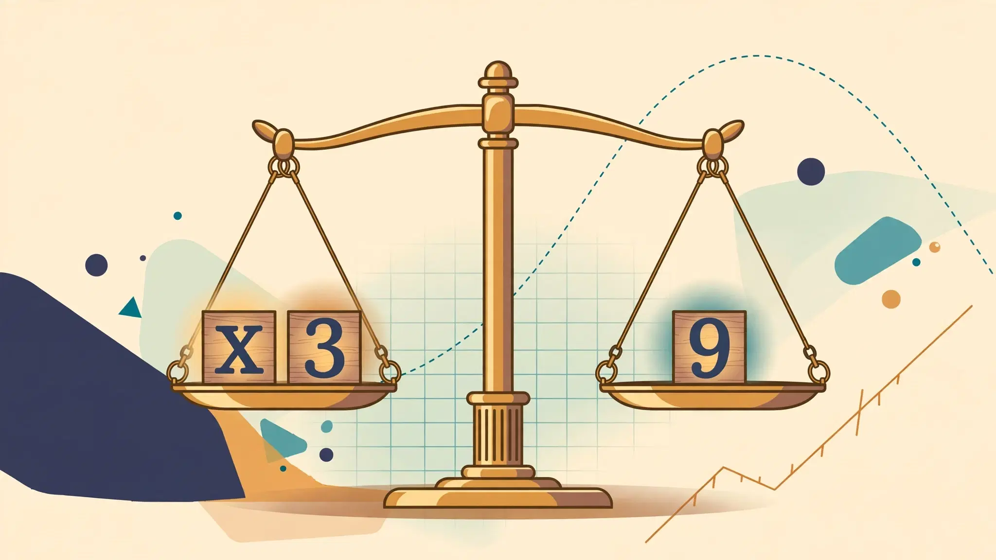
A quantity, multiplied by 1 and 1/2, plus 4, gives 10. What is the quantity? That puzzle, a first glimpse of how algebra works, comes from the Rhind papyrus, written in Egypt around 1650 BCE, and it is one of the oldest algebra problems we still have. The answer is 4, because 4 times 1.5 is 6, and 6 plus 4 is 10. Nobody in Egypt at the time wrote it with an x. They wrote it out in words, and they solved it by working backwards. Yet the thinking is exactly the thinking you use when you meet an equation today: a number is hidden, the clues around it are plain, and a few careful steps bring it into the open.
That is how algebra works, at its heart. It is the branch of mathematics that reasons with abstract symbols rather than specific numbers. Instead of calculating 2 + 3 = 5 and stopping there, algebra writes a letter where a number is missing, and then reasons about the relationship until the missing number shows itself. The letter looks small and quiet on the page. The idea behind it is enormous, because once you can write a relationship down in symbols, you can solve it, graph it, generalise it, and use the same pattern on a thousand problems that look different on the surface.
This article explains how algebra works from the ground up. You will learn the vocabulary, the balance rule that solves every equation in this article, linear equations and their straight-line graphs, systems of equations, functions, and quadratics with all four solving methods. You will then follow the history from Babylonian clay tablets to Baghdad, the cubic race in Italy, and the letters x, y and z. You will see why there is no general formula for the quintic, and you will finish with the mechanisms that make algebra useful in daily life: the four equations that find your position from satellites, the arithmetic that keeps secrets safe, the matrices that draw pictures and train machine learning, and the linear models behind distance, interest and recipes. Every worked calculation in this article has been checked, and the numbers are given exactly as worked. By the end, you should be able to solve a linear equation, solve a quadratic equation, read a graph, and explain to someone else why the same tool runs so much of the modern world.
1. What Algebra Really Is
Algebra is the branch of mathematics in which arithmetical operations and formal manipulations are applied to abstract symbols rather than specific numbers. That definition, from Encyclopaedia Britannica, draws the line in a useful place: arithmetic computes with numbers you already know, while algebra reasons with symbols that stand for numbers you do not yet know, or for numbers that can change. The Britannica page puts the distinction in a memorable way, and it is worth meeting early, because it clears up a confusion that follows many learners for years.
x + y = z or b - 2 = 5 are algebraic equations, but 2 + 3 = 5 and 73 times 46 = 3,358 are not. — Encyclopaedia Britannica, "Algebra | History, Definition, and Facts"
The first two statements contain letters, and the letters do work: they stand for numbers, and the statement claims a relationship between them. The last two contain only known numbers, so they are arithmetic, even though one of them is a long multiplication. The presence of a letter is not decoration. It is the whole point. When you write x + y = z, you are saying something that stays true for many choices of numbers at once, and you can ask what happens when one of them changes.
The shift from calculating answers to describing relationships is the first idea to hold on to. In arithmetic, the usual question is "what is the answer?" In algebra, the usual question is "what is the relationship, and what does it force the unknown to be?" A phone plan that charges a fixed amount plus a rate per minute is a relationship. A recipe that doubles when you double the servings is a relationship. A line on a graph is a relationship. Algebra gives you a compact language for writing those relationships down, and a set of moves for working with them.
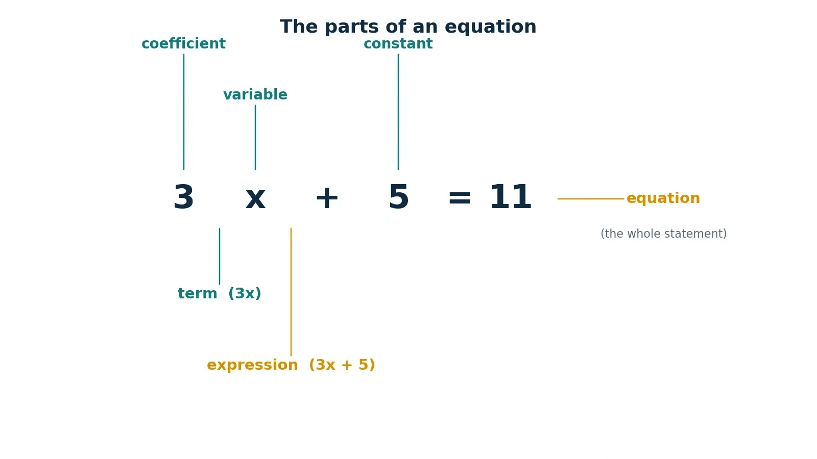
Here is the vocabulary, in one place, so the rest of the article can use it without stopping to explain each word again. A variable is a symbol, usually a letter such as x, y or z, that represents an unspecified value, either one unknown number to be found, or a quantity that can vary. A constant is a fixed number, or a symbol such as pi whose value does not change. A coefficient is the constant factor multiplying a variable in a term; in 3x, the coefficient is 3. A term is a single number, variable, or product of numbers and variables, for example 3x or 5. An expression is a combination of terms joined by addition or subtraction, for example 3x + 5; it has no equals sign. An equation is a statement that two expressions are equal, for example 3x + 5 = 11; it has an equals sign. These definitions come from OpenStax Intermediate Algebra, and they are the working definitions used throughout this article.
A first tiny example shows how algebra works in miniature. Take 2x + 6 = 14. Subtract 6 from both sides: 2x = 8. Divide both sides by 2: x = 4. Check by putting 4 back in: 2 times 4 + 6 = 14, which is correct. Nothing mysterious happened. Each step did the same thing to both sides, and the unknown was left standing alone. That pattern, repeated with more care and more steps, solves every linear equation in this article, and the same instinct, keeping the two sides equal while you reshape them, sits behind the quadratic methods too.
The modern concept of an equation as a single mathematical entity took until the late 16th century to consolidate. That is a useful fact to carry with you, because it explains why the idea feels both obvious and strange. The equation looks like a natural object now, a single thing you can move around and transform. For most of its history it was not treated that way. People solved problems one at a time, in words, with procedures fitted to each case. The shift to treating an equation as an object in its own right, something you can add to, multiply, factor and graph, was a slow achievement, and it is the achievement this article follows.
| Expression | Equation |
|---|---|
| A combination of terms, for example 3x + 5 | A statement that two expressions are equal, for example 3x + 5 = 11 |
| Has no equals sign | Has an equals sign |
| Can be simplified or evaluated, but not solved | Can be solved: a solution is a value that makes it a true statement |
| Example: 3x + 5, x squared + 2x - 3 | Example: 3x + 5 = 11, x squared + 2x - 3 = 0 |
The table above is the quickest reference in the article. If you are ever unsure whether you are looking at an expression or an equation, look for the equals sign. No equals sign means you have a phrase. An equals sign means you have a sentence that makes a claim, and a claim can be tested by substitution, which is how every check in this article works.
2. The Language of Unknowns: Variables, Expressions and Equations
Algebra explained in one sentence is this: it is the art of writing relationships with letters, and then using the rules of arithmetic on those letters to find out what the letters must be. The sentence sounds simple. The practice takes a little time, because reading algebra is a skill in itself, and it rewards the same patience you would give to learning to read music or a new alphabet. Each symbol has a job, and the jobs combine into sentences that say something precise.
Start with the variable, since it is the letter most people meet first and the one most often misunderstood. A variable is a symbol, usually a letter such as x, y or z, that represents an unspecified value. That value can play two different roles, and confusing them causes real trouble. Sometimes the variable is one unknown number to be found, as in 2x + 6 = 14, where x turns out to be 4 and nothing else. Sometimes the variable is a quantity that can vary, as in y = 2x + 3, where x can be 0, 1, 4, or any other number, and y changes with it. A variable is not always a mystery number with a single secret answer. It can also be a placeholder for a whole range of values, and much of algebra is about the second role, describing how one quantity changes when another changes.
That is why the correction to a common misconception belongs here, at the moment the reader first meets the idea: x does not always stand for one fixed mystery number. In an equation to be solved, it often does. In a formula or a function, it stands for something that varies, and the equation describes the pattern of that variation. If you read every x as a single hidden number, graphs and functions will look confusing, because a graph shows all the values at once. If you read every x as something that varies, solving a single equation will look confusing, because the answer is one value. The skill is to notice which role the letter is playing in the sentence you are reading.
An expression is a phrase. An equation is a sentence. That analogy helps more than it first seems. The expression 3x + 5 is like the phrase "three times a number, plus five": it names a quantity, but it claims nothing about it, and you cannot solve it. Add an equals sign and a number, 3x + 5 = 11, and you have a sentence that makes a claim: this quantity is 11. A claim can be true or false for a given value of x, and solving the equation means finding the values that make the claim true. A solution is a value that makes the equation a true statement, and the check at the end of every worked example in this article is simply putting the value back in and seeing whether the claim holds.
Polynomials are the most important family of expressions in school algebra, and they deserve a careful introduction. A polynomial is an expression consisting of variables and coefficients, using addition, subtraction and multiplication, with non-negative integer exponents only. That last condition is the one that draws the boundary: x squared is allowed, x to the power of one half is not a polynomial term, and one divided by x is not a polynomial term. Inside that boundary, polynomials are classified by how many terms they have. One term is a monomial, for example 5x squared. Two terms make a binomial, for example x + 3. Three terms make a trinomial, for example x squared + 2x - 3. The degree of a polynomial is the highest exponent in it, so x squared + 2x - 3 has degree 2, and 3x + 5 has degree 1. The degree turns out to be one of the most useful facts about a polynomial, because it tells you the shape of its graph and the maximum number of solutions its equation can have, as Section 8 shows.
| Type of polynomial | Number of terms | Example | Degree |
|---|---|---|---|
| Monomial | One term | 5x squared | 2 |
| Binomial | Two terms | x + 3 | 1 |
| Trinomial | Three terms | x squared + 2x - 3 | 2 |
| Polynomial, general | One or more terms | 3x + 5 | 1 |
The degree rule is simple to state and worth remembering now, because it returns in every later section. A linear equation has the highest power 1, its graph is a straight line, and it has at most one solution. A quadratic equation has the highest power 2, its graph is a parabola, and it has at most two real solutions. A cubic equation has the highest power 3, and it has at most three real solutions. The degree sets a ceiling on the number of solutions, and the discriminant in Section 9 tells you how many of those solutions are real in a given case.
The last point in this section is about the equals sign itself, and it leads directly into Section 3. In arithmetic, the equals sign often behaves like a button on a calculator: 2 + 3 = 5 reads as "work it out, and the answer is 5". In algebra, the equals sign means "is equal to", a statement that the two sides name the same quantity. That change of meaning is small on the page and large in the mind, and it is the hinge on which the whole subject turns.
3. Algebra Versus Arithmetic: Why Letters Change Everything
I still remember a classroom moment from years ago, when a student stared at 2x + 6 = 14 and said, quite reasonably, that the x was in the way. She could add and multiply without trouble. What bothered her was not the arithmetic but the letter itself, sitting where a number ought to be, refusing to be a number. I asked her what number she thought x might be, and she guessed 5, then 3, then 4, testing each one in her head. When she reached 4, her face changed, because 2 times 4 + 6 is 14, and the letter had stopped being an obstacle and started being a question with an answer. That moment is the whole subject in miniature: algebra is not arithmetic with letters glued on. It is a different kind of thinking, and the letter is the tool that makes it possible.
Arithmetic computes with specific numbers using the four operations. Algebra reasons about relationships and general rules. It uses letters for unknowns and for varying quantities, treats the equals sign as "is equal to" rather than "calculate now", and solves by transforming equations into equivalent equations, doing the same operation to both sides. That distinction, drawn from a discussion of algebra versus arithmetic, is the one to keep. Arithmetic asks for a value. Algebra asks for a pattern, and then uses the pattern to find values.
The misconception to name plainly is this: the equals sign means "calculate now". It is a natural reading, because that is how the sign is used in the first years of school. A child sees 2 + 3 = 5 and learns that the sign announces the answer. Then algebra arrives, and the sign starts appearing in the middle of a sentence, with unknowns on both sides, and the "calculate now" reading breaks down. In 2x + 6 = 14, there is nothing to calculate yet, because x is unknown. The sign is not an instruction. It is a claim that the two sides are equal, and the work of solving is to reshape the sentence, keeping the claim true, until x stands alone.
Try the contrast with two small problems. First, an arithmetic problem: 15 + blank = 40. The blank is 25, and you find it by subtraction. Second, an algebraic relationship: the first blank is 4 more than the second blank. That second statement does not pick out one pair of numbers. It describes a whole family of pairs: if the second blank is 1, the first is 5; if the second is 10, the first is 14; if the second is 100, the first is 104. The relationship stays the same while the numbers vary, and that is algebraic thinking. The first problem has an answer. The second has a rule, and the rule can generate answers without end.
Here is a short pair of problems to try yourself, with the answers given so you can check your thinking. Problem one: a number plus 9 is 23. What is the number? Write it as x + 9 = 23, subtract 9 from both sides, and x = 14. Problem two: a number is 7 more than another number, and the two numbers add to 31. What are they? Call the smaller number y, so the larger is y + 7, and y + (y + 7) = 31, which gives 2y + 7 = 31, 2y = 24, y = 12, and the larger number is 19. The first problem is one unknown and one clue. The second is two unknowns tied together by a relationship, and the relationship is what makes it solvable. That is the step from arithmetic to algebra, and it is how algebra works: you stop hunting for a single number and start writing down how quantities relate.
The balance rule, which Section 4 explains in full, is the practical form of relational thinking. Whatever operation is done to one side of an equation must be done to the other side, or the equality breaks. That is the single rule behind every solving method in this article, and it is the direct descendant of al-jabr and al-muqabala, the completion and balancing of al-Khwarizmi's book. The language of balance is not a metaphor added for charm. It is the literal history of the subject, and it is also the most reliable way to check your own work: if you would not do it to both pans of a scale, do not do it to one side of an equation.
4. The Balance Rule: How Algebra Works When You Solve an Equation
A tutoring memory comes back to me whenever I explain the balance rule. A student I was helping had learned the steps for solving linear equations, and she could repeat them, but she kept making the same mistake: she would subtract a number from one side and forget the other. I drew a balance scale on a piece of paper, with 2x + 6 on the left pan and 14 on the right, and I asked her what would happen if she took 6 off the left pan only. She laughed, because the picture made the answer obvious: the scale would tip, and the two sides would no longer be equal. From then on, every time she solved an equation, she pictured the scale, and the mistake stopped. The picture was doing the work that the rule, repeated in words, had not done. That is why this section starts with the scale and keeps returning to it.
The general strategy for solving a linear equation, from OpenStax Intermediate Algebra, has five steps, and they are worth learning in order, because they work on every linear equation in this article. First, simplify each side of the equation as much as possible, using the distributive property and combining like terms. Second, collect all the variable terms on one side. Third, collect all the constants on the other side. Fourth, make the coefficient of the variable 1 by dividing or multiplying both sides as needed. Fifth, check the answer by substituting it back into the original equation. The table below states the strategy in full.
| Step | What to do | Example with 2x + 6 = 14 |
|---|---|---|
| 1. Simplify each side | Remove brackets with the distributive law and combine like terms | Both sides are already simple |
| 2. Collect variable terms on one side | Add or subtract to move variable terms to one side | No variable term on the right to move |
| 3. Collect constants on the other side | Add or subtract to move constants away from the variable | Subtract 6 from both sides: 2x = 8 |
| 4. Make the coefficient 1 | Divide both sides by the coefficient, or multiply by its reciprocal | Divide both sides by 2: x = 4 |
| 5. Check by substitution | Put the value back into the original equation | 2 times 4 + 6 = 14, which is correct |
The strategy is a habit, not a ritual. On a simple equation you may do two steps at once without thinking about it, and that is fine. On a harder equation, with brackets and fractions and variable terms on both sides, the steps keep you from losing track of which side holds what. The check at the end is not optional decoration. It is the moment the equation tells you whether the claim is true, and it catches the small slips that even careful solvers make.
Now the worked examples, each done step by step with the check shown. First, the one-step example from Section 1, repeated here because it is the pattern all the others follow. Solve 2x + 6 = 14. Subtract 6 from both sides: 2x = 8. Divide by 2: x = 4. Check: 2 times 4 + 6 = 14. Correct. Second, a similar equation with a different shape. Solve 3x - 7 = 11. Add 7 to both sides: 3x = 18. Divide by 3: x = 6. Check: 3 times 6 - 7 = 11. Correct. In both cases, the move is the same: undo the addition or subtraction first, then undo the multiplication. The order matters, because it reverses the order in which the expression was built: the expression 2x + 6 was built by multiplying by 2 and then adding 6, so solving undoes the adding first and the multiplying second.
Third, a problem from the Rhind papyrus, around 1650 BCE, solved with the same method the Egyptians used in words. Solve (3/2)x + 4 = 10. Subtract 4 from both sides: (3/2)x = 6. Multiply both sides by 2/3: x = 4. Check: 4 times 1.5 is 6, plus 4 is 10. Correct. The fraction looks more difficult than the whole numbers, but the moves are identical: subtract the constant, then deal with the coefficient. Multiplying by the reciprocal 2/3 is the same as dividing by 3/2, and it is worth getting comfortable with, because coefficients in real problems are often fractions.
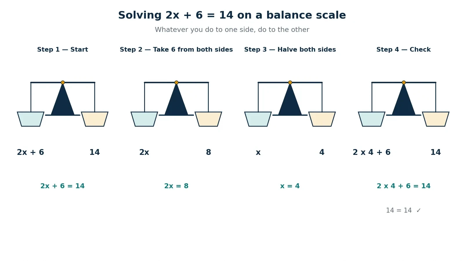
The figure above shows those steps as a scale, one pan per step, and it is worth studying slowly. In the first panel, the scale is balanced with 2x + 6 on the left and 14 on the right. In the second, 6 is removed from both pans, and the scale stays balanced with 2x = 8. In the third, both pans are halved, and the scale shows x = 4. The last panel is the check, putting 4 back in and confirming that both sides are 14. Nothing in the picture is a trick. Every move keeps the scale level, and that is the whole rule: whatever you do to one side, do to the other.
Not every equation has a single answer, and the three kinds are part of how algebra works. A conditional equation is true for one or more values of the variable. The example from OpenStax is 7x + 8 = -13, which is true when x = -3, because 7 times -3 is -21, and -21 + 8 is -13. An identity is true for every value of the variable. The example is 7y + 14 = 7(y + 2): expand the right side with the distributive law and you get 7y + 14 on both sides, so every value of y works, and there is no single answer to find. A contradiction is false for every value of the variable and has no solution. The example is -8z = -8z + 9, which leads to 0 = 9 after adding 8z to both sides, and 0 = 9 is false, so no value of z can satisfy it. When you meet an equation that simplifies to a true statement with no variable left, such as 14 = 14, you have an identity. When it simplifies to a false statement with no variable left, such as 0 = 9, you have a contradiction. Neither is a mistake. Both are answers of a different kind: the first says every number works, the second says no number works.
5. Linear Equations and Straight Lines
A linear equation in one variable can be written in the form a x + b = 0, where a and b are real numbers and a is not 0. That definition, from OpenStax, is deliberately plain, and its plainness is the point: a linear equation is the simplest kind of equation, one in which the variable appears only to the first power, with no squares, no roots and no fractions involving the variable. Its graph is a straight line. That single fact connects the algebra of solving to the geometry of drawing, and it is the first place where the two subjects meet in this article. They will meet again, more deeply, in Section 12, with Descartes.
The straight line has its own language, and it is worth learning carefully, because lines are the picture of linear relationships. The slope-intercept form of a line is y = m x + b, where m is the slope and b is the y-intercept, the point where the line crosses the y-axis, at x = 0. The point-slope form is y - y1 = m (x - x1), for a line of slope m through the point (x1, y1). The slope between two points (x1, y1) and (x2, y2) is (y2 - y1) divided by (x2 - x1). Those three formulas, from OpenStax Intermediate Algebra section 3.3, are the whole toolkit for lines, and each one answers a different question: slope-intercept form is best when you know the slope and where the line crosses the y-axis; point-slope form is best when you know the slope and one point the line passes through.
Take the line y = 2x + 3 and work with it slowly, because it is the example this article returns to again and again. The slope m is 2, and the y-intercept b is 3. That means the line crosses the y-axis at the point (0, 3), and for every step of 1 to the right, it rises 2. The points confirm it: when x = 0, y = 3; when x = 1, y = 5; when x = 4, y = 11. The slope between (1, 5) and (4, 11) is (11 - 5) divided by (4 - 1), which is 6 divided by 3, which is 2, matching the slope in the equation. The check is not a formality. It shows that the number in the equation and the steepness of the drawn line are the same thing, seen two ways.
A second line makes the contrast clear. The line through (0, -4) with slope -9 is y = -9x - 4. At x = 1, y = -13, because -9 times 1 is -9, and -9 - 4 is -13. The negative slope means the line falls as x increases, steeply, nine units down for every unit across. Put the two lines side by side in your mind: y = 2x + 3 climbs gently to the right, crossing the y-axis above the origin, while y = -9x - 4 plunges downward, crossing the y-axis below the origin. The sign of the slope tells you the direction. The size of the slope tells you the steepness. The intercept tells you where the line starts on the y-axis. Three numbers, and you can picture the line before you draw it.
Point-slope form earns its place when you know a point and a slope but not the intercept. Take the line with slope -2 through the point (-1, 3). Point-slope form gives y - 3 = -2(x + 1). Expand the right side: y - 3 = -2x - 2. Add 3 to both sides: y = -2x + 1. Now the line is in slope-intercept form, and you can read off the slope -2 and the intercept 1. Check with points: at x = 0, y = 1; at x = 2, y = -3, because -4 + 1 is -3. The line passes through (-1, 3) as promised, because -2 times -1 is 2, and 2 + 1 is 3. Point-slope form is a bridge: it takes you from what you know, a point and a slope, to what you want, the full equation of the line.
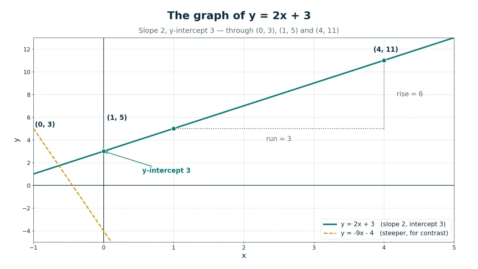
The graph above shows y = 2x + 3 with its points marked, and a steeper line for contrast. Study the slope triangle between (1, 5) and (4, 11): the run is 3, the rise is 6, and 6 divided by 3 is 2, the slope. A slope is a ratio, rise divided by run, and the triangle makes that ratio visible. If the triangle is wide and flat, the slope is small. If it is tall and narrow, the slope is large. Drawing the triangle is a good habit whenever a slope feels abstract, because it turns a number into a shape you can see.
| Form | Equation | Best when you know | What you read off directly |
|---|---|---|---|
| Slope-intercept | y = m x + b | The slope and the y-intercept | Slope m and intercept b |
| Point-slope | y - y1 = m (x - x1) | The slope and one point (x1, y1) | Slope m and the point (x1, y1) |
That movement between algebra and geometry is the thread that runs through the rest of the article. A system of equations is two lines and the question of where they meet. A function is a rule and the curve it draws. A quadratic is a parabola and the question of where it crosses the x-axis. Each time, the equation tells you the rule, and the graph shows you all the answers at once. Learning to read both, and to check one against the other, is what it means to understand how algebra works, rather than merely to carry out its steps.
6. Systems of Equations: When One Equation Is Not Enough
One equation can find one unknown. Two unknowns need two equations, and that simple fact is the whole idea of a system of equations. A single equation with two unknowns, such as x + y = 10, has infinitely many solutions: x could be 1 and y 9, or x could be 6 and y 4, or x could be 10 and y 0, and each pair satisfies the equation. Add a second equation, x - y = 2, and the freedom collapses: only one pair satisfies both at once. That pair is the solution of the system, and finding it is how algebra works with more than one unknown: use the two equations together so that one unknown disappears and the other can be found.
There are three ways to solve a system, and each one is useful in a different situation. Graphing means drawing both lines and looking for where they cross, which is the point that satisfies both equations. Substitution means solving one equation for one variable and putting that expression into the other equation, so the second equation has only one unknown left. Elimination means adding or subtracting the equations so that one variable cancels, leaving a single equation in the other variable. A system has one solution if the lines intersect once, no solution if they are parallel, and infinitely many solutions if they are the same line. Those three outcomes are the whole story, and they are visible on a graph before any algebra is done: crossing lines, parallel lines, and coincident lines.
Work the first system by elimination, because it is the cleanest example. Solve x + y = 10 and x - y = 2. Add the two equations: the y terms cancel, because y plus -y is 0, and the left sides add to 2x while the right sides add to 12. So 2x = 12, and x = 6. Put x = 6 into the first equation: 6 + y = 10, so y = 4. Check both equations: 6 + 4 = 10, and 6 - 4 = 2. Correct. The elimination step did the work by making one variable vanish, and the rest was a single linear equation of the kind Section 4 taught.
Work a second system by substitution, to show the other method in action. Solve 2x + 3y = 12 and x - y = 1. From the second equation, x = y + 1. Substitute that into the first equation: 2(y + 1) + 3y = 12. Expand: 2y + 2 + 3y = 12, so 5y + 2 = 12, 5y = 10, and y = 2. Then x = y + 1 = 3. Check both equations: 2 times 3 + 3 times 2 is 6 + 6, which is 12, and 3 - 2 is 1. Correct. Substitution is the better choice when one equation already has a variable nearly alone, as the second equation did here. Elimination is the better choice when the coefficients line up so that adding or subtracting cancels a variable at once, as in the first system. Graphing is the better choice when you want to see what is happening, or when the numbers are simple enough to read off the picture.
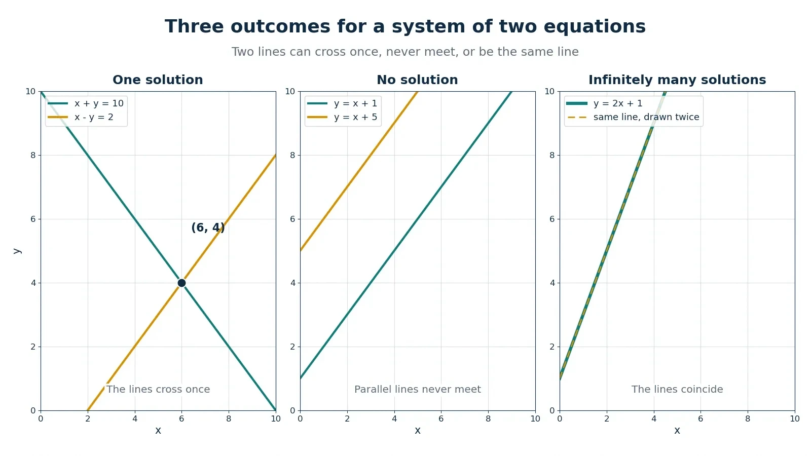
The figure above shows all three outcomes side by side. In the first panel, the lines x + y = 10 and x - y = 2 cross at (6, 4), the solution just found. In the second panel, two parallel lines never meet, so the system has no solution: the equations contradict each other, and no pair can satisfy both. In the third panel, two lines lie exactly on top of each other, so every point on the line is a solution, and the system has infinitely many. The picture is a check on the algebra: if your algebra says there is one solution, the lines should cross once; if it says there is none, they should be parallel; if it says there are infinitely many, they should coincide. When the picture and the algebra disagree, one of them has an error, and the disagreement is worth investigating.
Systems are not a classroom exercise with no life outside the page. A GPS receiver, as Section 14 explains in detail, solves for four unknowns, its x, y and z position and its own clock error, so it needs signals from at least four satellites, each satellite giving one distance equation. The two-equation system in this section is a miniature of that problem: two unknowns, two equations, one answer. The step from two equations to four is a step of size, not of kind, and the elimination idea scales up with it: subtract equations pairwise to cancel the squared terms and leave a linear system, then solve. If you want the full story now, the article on how GPS works carries it through with satellites and atomic clocks, and it is worth reading alongside this section.
7. Functions: Machines That Turn Inputs into Outputs
A function is a rule that assigns each input exactly one output. That definition is short, and it carries the whole idea. The inputs form a set called the domain. The outputs form a set called the range. The function is written f(x), read as "f of x", where x is the input and f(x) is the output. The example that runs through this section is f(x) = 2x + 3, the same line from Section 5, now seen as a machine: put a number in, double it, add three, and the result comes out. The values are f(0) = 3, f(1) = 5 and f(4) = 11, the same points that lay on the line, because a function and its graph are two views of the same rule.
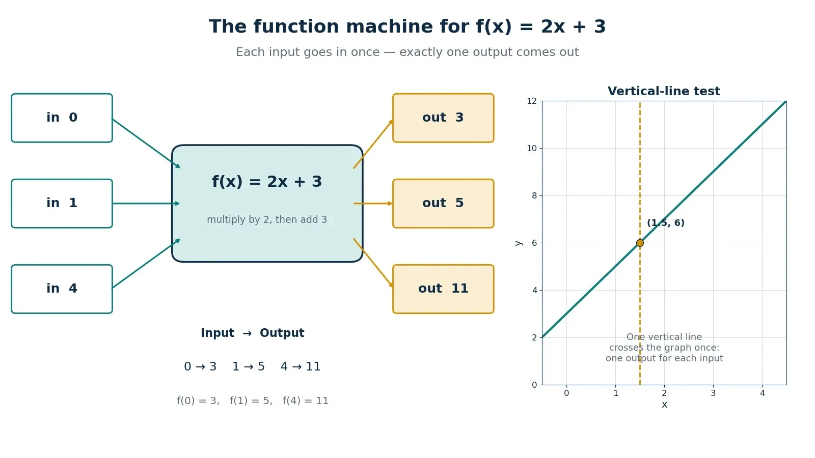
Here is the input-output table for f(x) = 2x + 3, laid out plainly so the pattern is visible. When the input is 0, the output is 3. When the input is 1, the output is 5. When the input is 4, the output is 11. Each input appears once, and each has one output. The table is small, but it shows the structure: a function is a table with no repeated input, a rule that never contradicts itself. You can extend the table as far as you like, to negative inputs, to fractions, to any number at all, and the rule keeps working, because doubling and adding three are operations that work on any number.
Functions matter beyond their definition because they are the objects that the rest of mathematics studies. Calculus, in particular, studies functions: how fast they change, how much they accumulate, where they reach their highest and lowest values. The article on how calculus works takes up that story, and it is worth reading after this section, because it shows what happens when you ask not just "what is the output for this input?" but "how is the output changing as the input changes?" That second question is the beginning of calculus, and it is built entirely on the idea of a function introduced here. A line, a parabola, a wave and a growth curve are all functions, or pieces of functions, and the tools for studying them all start with the definition in this section.
The most common confusion is between a function and a relation that is not a function. A relation is any pairing of inputs and outputs. A function is a relation with the extra rule that each input has exactly one output. The circle is a relation but not a function. The equation x squared + y squared = 25 describes a circle, and for x = 0 it gives y = 5 and y = -5, two outputs for one input. The equation y = 2x + 3 describes a line, and for x = 0 it gives only y = 3, one output. The difference is not about how complicated the equation looks. It is about whether the rule gives a single answer for each input, and that is a question you can test with the vertical line or with a table.
8. Quadratics: When the Unknown Is Squared
A quadratic equation is an equation that can be written in standard form a x squared + b x + c = 0, where a is not 0. Its graph is a parabola, a U-shaped curve, and the word quadratic comes from Latin quadratus, meaning square, because the highest power is a square. The condition that a is not 0 is essential: if a were 0, the squared term would vanish, and the equation would be linear, not quadratic. The standard form is the starting point for every solving method in Section 9, so it is worth learning to recognise it at a glance, even when an equation is written in a different order or with terms on both sides.
Work with the example y = x squared - 4x + 3, the parabola this section studies in detail. The vertex x-coordinate is -b divided by (2a), which is 4 divided by 2, which is 2. The y value at x = 2 is 4 - 8 + 3, which is -1. So the vertex is (2, -1), the lowest point of the curve, and the axis of symmetry is the vertical line x = 2. The roots are x = 1 and x = 3, because (x - 1)(x - 3) expands to x squared - 4x + 3, and the parabola crosses the x-axis at those two points. The y-intercept is 3, because at x = 0 the value is 3. Put those landmarks together and the curve is fully described: it comes down from the left, touches its lowest point at (2, -1), and rises again, crossing the x-axis at 1 and 3 and the y-axis at 3.
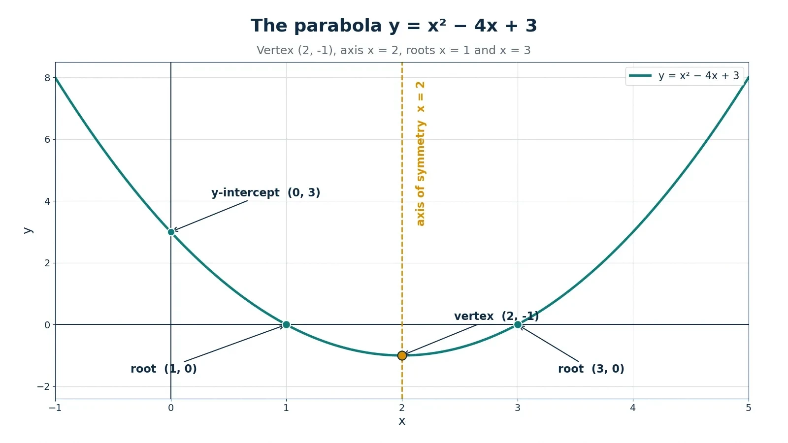
A projectile gives a concrete picture of a parabola in motion, and the model in this article is labelled as a model, not as a measured throw. Suppose the height h of a thrown object, in metres, follows h = -5 t squared + 20 t, where t is time in seconds. The coefficient -5 is a rounded stand-in for half of gravitational acceleration in metres per second squared, and the article states that plainly rather than presenting it as an exact physics constant. At t = 2, h = -20 + 40 = 20, so the object is 20 metres up after two seconds. At t = 4, h = -80 + 80 = 0, so it has returned to the ground after four seconds. The vertex is at t = 2, height 20, which is the highest point of the flight. The model is simple, and its simplicity is the point: the same quadratic shape that describes a parabola on paper describes the arc of a throw, and the vertex of the curve is the top of the arc.
| Type | Highest power | Graph shape | Maximum real solutions |
|---|---|---|---|
| Linear | 1 | Straight line | 1 |
| Quadratic | 2 | Parabola | 2 |
| Cubic | 3 | Curve with up to two turns | 3 |
The table above gathers the degree rule from Section 2 into one place. A linear equation has at most one solution, a quadratic at most two, a cubic at most three. The word "at most" matters: a quadratic can have two solutions, one solution, or no real solutions, depending on its discriminant, and Section 9 works through all three cases. A parabola that sits entirely above the x-axis never crosses it, and its equation has no real roots. A parabola that just touches the x-axis has one repeated root. A parabola that crosses twice has two distinct roots. The graph and the discriminant tell the same story, and the next section shows how to read it, which is part of how algebra works.
9. Solving Quadratics: Factoring, Completing the Square, and the Formula
There are four methods for solving a quadratic equation, and each one is quickest in a different situation. Factoring is quickest when the quadratic splits neatly into two brackets with whole numbers. The square-root property is quickest when the equation has no x term, or when it is already a perfect square equal to a number. Completing the square is the method that always works, and it is the method the quadratic formula is built from. The quadratic formula is the universal tool: it works on every quadratic, and it tells you at a glance, from the discriminant, how many real solutions there are. Learning all four matters for understanding how algebra works, because the fast method saves time when it applies, and the universal method saves you when it does not.
Factoring rests on the zero-product property: if a product equals zero, at least one factor is zero. That is why factoring solves equations: once a quadratic is written as a product equal to zero, each factor can be set equal to zero in turn. Take x squared - 5x + 6 = 0. It factors as (x - 2)(x - 3) = 0, so x = 2 or x = 3. Check both: 4 - 10 + 6 = 0, and 9 - 15 + 6 = 0. Correct. Take a second example, x squared + 7x + 12 = 0. It factors as (x + 3)(x + 4) = 0, so x = -3 or x = -4. Check both: 9 - 21 + 12 = 0, and 16 - 28 + 12 = 0. Correct. In each case, the factoring step turns one quadratic equation into two linear ones, and each linear equation gives one root. The skill in factoring is finding the two numbers that multiply to the constant term and add to the coefficient of x, and it comes with practice.
The square-root property is the second method, and it is the quickest when an equation is already a perfect square equal to a number. If a square equals a number, the thing squared equals the positive or the negative square root of that number. Take (x + 3) squared = 16. Then x + 3 = 4 or x + 3 = -4, so x = 1 or x = -7. Check both: (1 + 3) squared is 16, and (-7 + 3) squared is also 16. Correct. The two signs are the whole point: a square forgets whether its root was positive or negative, so solving must restore both.
Completing the square is the geometric idea behind the formula, and it deserves to be worked slowly at least once. Take x squared + 6x + 5 = 0. Move the 5 to the other side: x squared + 6x = -5. Add (6/2) squared, which is 9, to both sides: (x + 3) squared = 4. Take the square root of both sides, remembering both signs: x + 3 = 2 or x + 3 = -2, giving x = -1 or x = -5. Check both: 1 - 6 + 5 = 0, and 25 - 30 + 5 = 0. Correct. A second example: x squared + 6x - 7 = 0 gives (x + 3) squared = 16, so x = 1 or x = -7. Check both: 1 + 6 - 7 = 0, and 49 - 42 - 7 = 0. Correct. The name describes the picture: adding 9 completes a square of side x + 3, turning a lopsided expression into a perfect square plus a number. It is the same move al-Khwarizmi made geometrically on a literal square, as Section 12 shows, and it is the move that, done once in general with letters instead of numbers, gives the quadratic formula.
The quadratic formula is completing the square done once, in general. For a x squared + b x + c = 0, with a not 0, x equals -b plus or minus the square root of (b squared - 4 a c), all divided by (2a). The quantity under the square root, b squared - 4 a c, is called the discriminant, written D, and it decides how many real solutions there are before you finish the calculation. If D is positive, there are two distinct real solutions. If D is zero, there is one real solution, a repeated root. If D is negative, there are no real solutions, only two complex ones. The formula is stated and derived step by step in the LibreTexts page on solving quadratics with the quadratic formula, and that derivation is the place to go if you want to see completing the square carried out with a, b and c in place of numbers.
Work three examples by the formula, one for each discriminant case, so the rule is tied to numbers. First, x squared + 5x + 6 = 0, with a = 1, b = 5, c = 6. The discriminant is 25 - 24 = 1, and its square root is 1. So x = (-5 plus or minus 1) divided by 2, which is -2 or -3. Check both: 4 - 10 + 6 = 0, and 9 - 15 + 6 = 0. Correct. Second, the textbook example 2x squared + 9x - 5 = 0, with a = 2, b = 9, c = -5. The discriminant is 81 - 4 times 2 times (-5), which is 81 + 40 = 121, and its square root is 11. So x = (-9 plus or minus 11) divided by 4, which is 0.5 or -5. Check both: 2 times 0.25 + 9 times 0.5 - 5 = 0, and 2 times 25 - 45 - 5 = 0. Correct. Third, an example with fractions: 3y squared - 5y + 2 = 0. The discriminant is 25 - 24 = 1. So y = (5 plus or minus 1) divided by 6, which is 1 or 2/3. Check both: 3 - 5 + 2 = 0, and 3 times (4/9) - 5 times (2/3) + 2 = 0 exactly. Correct.
Now the two remaining discriminant cases, which correct a common misconception: a quadratic does not always have two answers. Take 4x squared - 20x + 25 = 0. The discriminant is 400 - 400 = 0, so there is one repeated root: x = 20 divided by 8 = 2.5, and the parabola touches the x-axis once. Check: 4 times 6.25 - 50 + 25 = 0. Correct. Take 3p squared + 2p + 9 = 0. The discriminant is 4 - 108 = -104, which is negative, so there are no real solutions. The parabola sits entirely above the x-axis and never crosses it. Those two cases are not failures of the method. They are answers: one solution, and no real solutions, are both possible, and the discriminant tells you which one you have before you take a square root.
| Discriminant D = b squared - 4 a c | Number of real solutions | Worked example |
|---|---|---|
| Positive, D = 121 | Two distinct real solutions | 2x squared + 9x - 5 = 0 gives x = 0.5 or x = -5 |
| Zero, D = 0 | One real solution, a repeated root | 4x squared - 20x + 25 = 0 gives x = 2.5 |
| Negative, D = -104 | No real solutions, two complex solutions | 3p squared + 2p + 9 = 0 has no real solutions |
I remember a puzzle that taught me to love the discriminant, though I did not know its name at the time. Someone asked me to find two numbers that add to 10 and multiply to 9, and I tried pairs until I found 9 and 1. Years later I learned that Diophantus had solved the same kind of problem, and that the discriminant is the test that tells you in advance whether such a pair exists. The puzzle is small, but the lesson is large: a formula is not just a machine for answers. It is also a test that tells you what kind of answer to expect, and that test can save you from hunting for a solution that does not exist.
10. Inequalities, Exponents and the Rest of the Toolkit
Inequalities, exponents and the distributive law are the supporting tools the earlier sections rely on, and this section gathers them in one place so they can be used without hesitation. An inequality is a statement that one quantity is greater than, or less than, another, and it is solved much like an equation, with one crucial difference: when you multiply or divide both sides by a negative number, the inequality sign flips. That flip is the one new rule, and it is the one that causes most mistakes, so it is worth working through carefully.
Take 2x + 3 is less than 11. Subtract 3 from both sides: 2x is less than 8. Divide by 2: x is less than 4. The sign does not flip, because 2 is positive. Now take -3x + 9 is greater than 0. Subtract 9 from both sides: -3x is greater than -9. Divide by -3, and the sign flips: x is less than 3. Check with numbers: x = 2 gives -6 + 9 = 3, which is greater than 0, true; x = 4 gives -12 + 9 = -3, which is not greater than 0, false. The check confirms the flip: without it, the answer would claim that numbers greater than 3 satisfy the inequality, and the test at x = 4 shows they do not. The balance rule still applies, doing the same thing to both sides, but the direction of the comparison reverses when both sides are multiplied or divided by a negative number, because multiplying by a negative reverses order on the number line.
| Exponent law | Rule in words | Numeric check |
|---|---|---|
| Multiplying powers, same base | Add the exponents | 2 cubed times 2 squared = 2 to the power 5 = 32 |
| Raising a power to a power | Multiply the exponents | (x squared) cubed = x to the power 6; at x = 2, both sides are 64 |
| Distributive law | Multiply each term inside the brackets | 3(x + 4) = 3x + 12; at x = 5, both sides are 27 |
Formulas in science are often linear equations in disguise, and rearranging them uses exactly the tools in this article. The pH scale, for example, is built around a formula that relates a measured quantity to its scale value, and the article on what the pH scale is shows how a single formula can turn a measurement into a number on a scale. The point for this section is not the chemistry but the algebra: a formula is an equation, and solving it for a different variable is the same balance-rule work as solving 2x + 6 = 14, with more letters and the same moves. Balancing a chemical equation, where the same number of each atom must appear on both sides, is a close cousin of the same idea, and the article on stoichiometry explains proportions and balancing in that setting. The algebra does not change when the subject changes, and that stability is how algebra works across the sciences. The letters stand for different quantities, and the moves stay the same.
11. A Short History of Algebra, Part 1: Babylon, Egypt, Greece and India
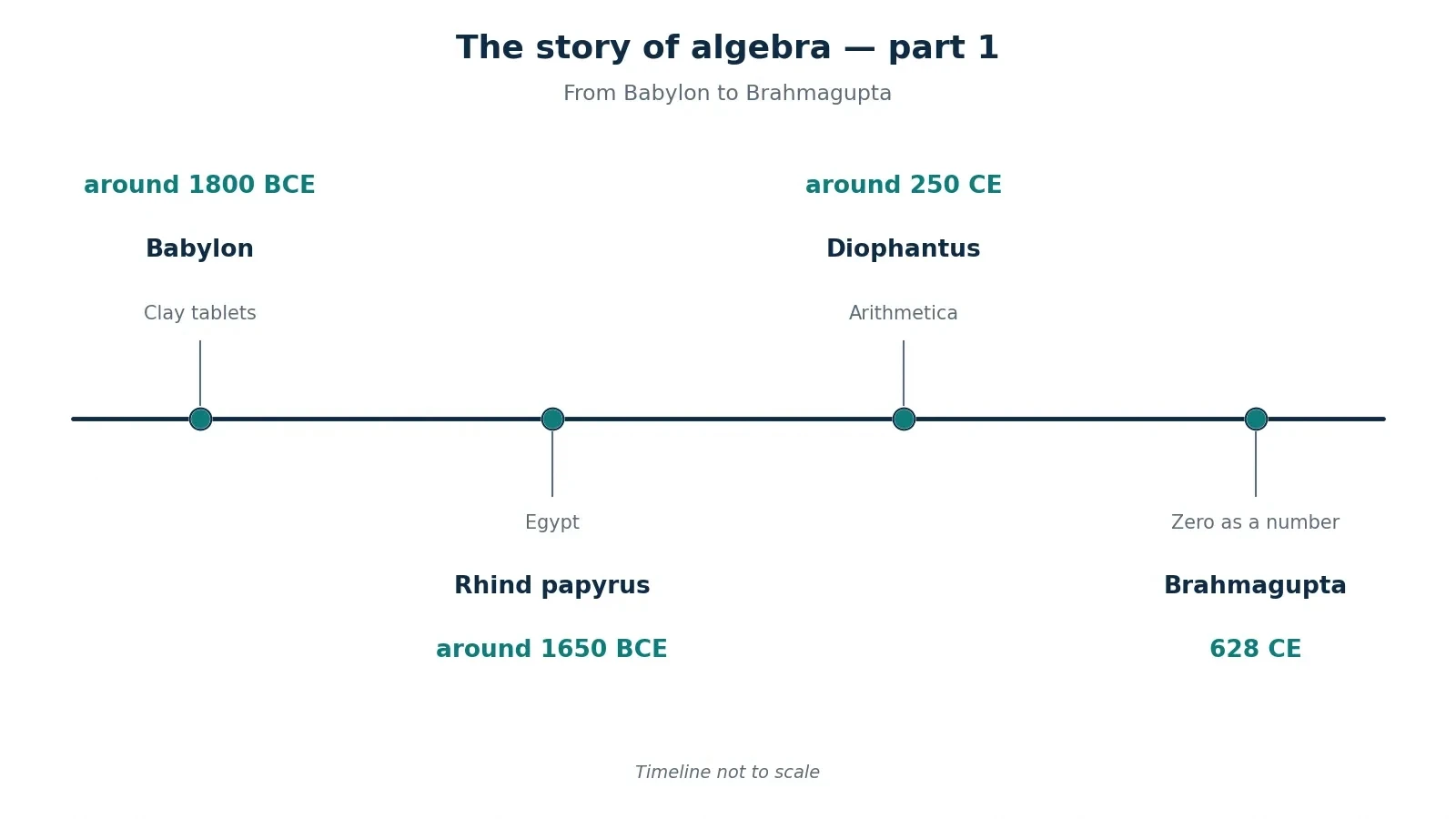
Algebra began as a collection of problems, not as a subject with a name. Babylonian mathematics dates from as early as 1800 BCE, from cuneiform clay tablets, and it used a positional sexagesimal system, base 60, to solve linear and quadratic problems by stated procedures for specific problems, not by general algorithms. It made no consistent use of zero. The Plimpton 322 tablet, from around 1900-1600 BCE, tabulates Pythagorean triples, which are sets of whole numbers that fit the rule for a right-angled triangle. The Babylonians could solve the problems they met. What they did not have was a general method written in symbols, so each problem needed its own procedure.
Egypt worked in words. The Rhind papyrus, from around 1650 BCE, is the earliest surviving Egyptian mathematical text, and it shows Egyptians solving linear equations in one unknown, stated and solved verbally, with no symbols. Its example is the puzzle that opened this article: a quantity, multiplied by 1 and 1/2, plus 4, gives 10, and the quantity is 4. By around 300 BCE Egyptians could also solve a system of two equations in two unknowns, including quadratics: a rectangle with perimeter 100 and area 600 has length 30 and width 20, because 2 times 30 + 2 times 20 = 100, and 30 times 20 = 600. The problems were practical, about land and quantities, and the solutions were recipes in words.
Diophantus of Alexandria, who flourished around 250 CE, took the first step from words toward symbols. The exact dates are debated: the only firm bounds are after 150 BCE and before 350 CE, and the date around 250 CE rests on a disputed reading of a letter, so this article gives it as a conventional estimate, not a certainty. His Arithmetica, in thirteen books, of which six survive in Greek and four more were found in an Arabic translation in Mashhad, Iran, in 1968, so ten of thirteen are now known, contains about 130 problems in the collection as described on the MacTutor page. He used abbreviations for the unknown and its powers, the first step from verbal toward symbolic algebra, but he had notation for only one unknown and no symbol for zero or for negative numbers. He called an equation leading to a negative answer "absurd", a vivid reminder of how strange negative numbers once seemed.
His worked example shows his method. Solve y + z = 10 and y z = 9. Put 2x = y - z, so y = 5 + x and z = 5 - x. Then 9 = (5 + x)(5 - x) = 25 - x squared, so x squared = 16, x = 4, giving y = 9 and z = 1. Check: 9 + 1 = 10, and 9 times 1 = 9. He also found that x = 28 makes both 10x + 9 and 5x + 4 into squares: 289 is 17 squared, and 144 is 12 squared, since 10 times 28 + 9 = 289 and 5 times 28 + 4 = 144. The details are recorded in the MacTutor biography of Diophantus, which also carries the debate about his dates.
Brahmagupta, from around 598 to around 668 CE, brought zero and negative numbers into algebra. His Brahmasphutasiddhanta, composed in 628 CE when he was about 30, is the earliest known text to treat zero as a number in its own right, with rules for addition, subtraction and multiplication with zero and with negative numbers. Positives were "fortunes" and negatives were "debts": a debt times a debt is a fortune, which is to say a negative times a negative is positive. He also gave the first clear description of the quadratic formula and solved general quadratic equations, accepting negative roots. His one error was stating that zero divided by zero is zero. He also worked on equations of the form N x squared + 1 = y squared, and solved the case N = 92 with x = 120 and y = 1151: 92 times 120 squared + 1 = 1,324,801, and 1151 squared = 1,324,801. Aryabhata is sometimes mentioned in this period, but the year 499 CE for his work on zero rests on a single secondary source that was not verified in this article's research, so he is left out here rather than stated as fact.
These stages have names. Rhetorical algebra means equations written in full sentences, used by the Babylonians and dominant until the 16th century. Syncopated algebra means some abbreviations, first in Diophantus in the 3rd century CE, then in Brahmagupta in the 7th century. Symbolic algebra means full symbolism, developed by Viete in the 16th century, with modern notation from Descartes in the 17th. The story so far has moved from the first stage into the second. The next section completes the move into the third.
The history of algebra is the history of a language learning to write itself down: first in sentences, then in abbreviations, and only at last in symbols that can be moved like pieces on a board.
12. A Short History of Algebra, Part 2: Baghdad, the Cubic Race, and the Letter x
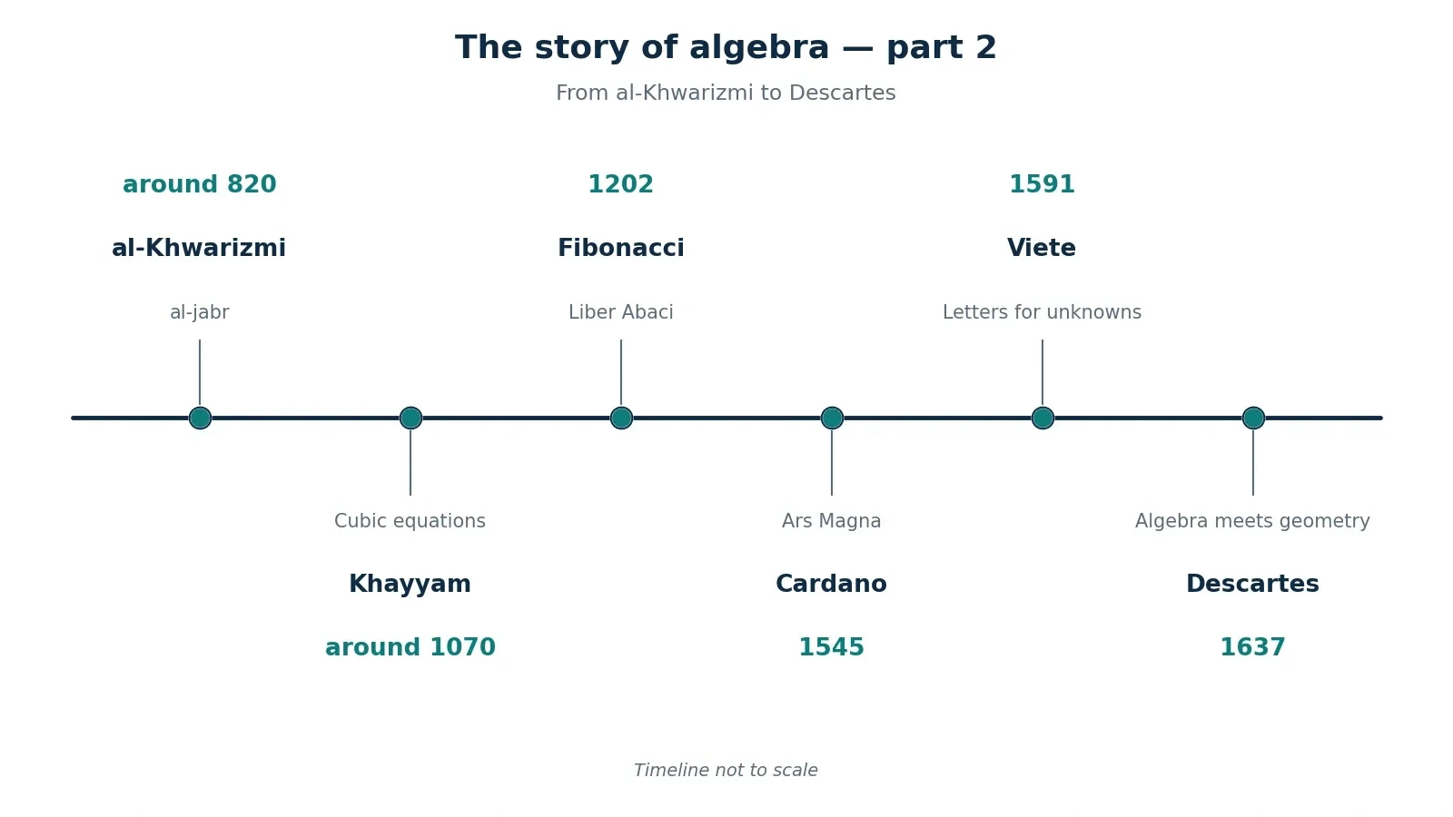
Al-Khwarizmi, from around 780 to around 850 CE, worked at the House of Wisdom in Baghdad under Caliph al-Mamun, who reigned 813-833. His book al-Kitab al-mukhtasar fi hisab al-jabr wal-muqabala, "The Compendious Book on Calculation by Completion and Balancing", written around 820 CE, was the first text to teach elementary algebra and the first to teach algebra for its own sake. It gave a systematic solution of linear and quadratic equations and reduced every case to six standard types. It was translated into Latin by Robert of Chester in 1145 and used as the principal mathematical textbook of European universities until the 16th century. The book's date is given as around 820 CE because sources differ: most say around 820, while one summary says 830, so no single exact year is stated as certain here.
The word algebra comes from Arabic al-jabr in that book's title. Al-jabr means restoration, completion, or "reunion of broken parts", the same root used for setting a broken bone. In an equation it means moving a subtracted term to the other side by adding it to both sides: 4x - 6 = 10 becomes, by al-jabr, 4x = 16. Al-muqabala means balancing: cancelling equal quantities on both sides. His name, Latinised as Algoritmi, "Al-Khwarizmi said", is the origin of the word algorithm. The balance rule of Section 4 is the direct descendant of those two words, and the connection is not decorative: the subject is named for the move that solves its equations.
His worked example is completing the square, done geometrically on a literal square. Solve x squared + 10x = 39. Halve 10 to get 5, square it to get 25, add to 39 to get 64, take the square root, 8, and subtract 5 to get 3. Check: 3 squared + 10 times 3 = 9 + 30 = 39. The method is the same one Section 9 teaches with numbers, and the picture behind it is a square being completed by adding a piece to its corner, which is where the name comes from.
Omar Khayyam, 1048-1131, wrote his Treatise on Demonstration of Problems of Algebra around 1070 CE in Samarkand. It was the first systematic classification of cubic equations, fourteen types with positive coefficients, solved geometrically by intersecting conic sections, a parabola with a circle, or a hyperbola with a circle. He realised a cubic can have more than one solution, and he said he had not found an algebraic formula for the root and that perhaps someone later would. His example, the cubic x cubed + 200x = 20x squared + 2000, was solved by intersecting a hyperbola with a circle. The formula he could not find arrived nearly five centuries later, in Italy.
Fibonacci, Leonardo of Pisa, published Liber Abaci in 1202 and revised it in 1228. It introduced Hindu-Arabic numerals and al-Khwarizmi's algebraic methods to Europe, and its final chapter discusses quadratic equations. The Fibonacci sequence 1, 1, 2, 3, 5, 8, 13, 21, 34, 55 appears in it, and the first ten terms add to 143. The ratio of successive terms approaches phi, which is (1 + the square root of 5) divided by 2, about 1.618, and phi squared equals phi + 1, both about 2.618. The article on the golden ratio and Fibonacci numbers carries that pattern into nature and art, and it is worth reading beside this section. For the history of pi itself, a constant that appears in the vocabulary of Section 1, see the article on pi explained.
Then came the cubic race. Scipione del Ferro found the solution of the depressed cubic x cubed + p x = q around 1515, though some sources say around 1505, so the date is disputed, and he did not publish it. Niccolo Tartaglia, born 1499/1500 and died 1557, solved it on 12 February 1535, eight days before a contest deadline against del Ferro's pupil Fior, and disclosed the method to Girolamo Cardano, 1501-1576, on 25 March 1539 after Cardano swore an oath not to publish it. Cardano published the cubic and quartic solutions in Ars Magna in 1545, crediting Tartaglia and del Ferro, and the quartic solution was by Cardano's pupil Ludovico Ferrari, 1522-1565. In Ars Magna, Cardano also made the first calculation with complex numbers, multiplying (5 + the square root of -15) by (5 - the square root of -15) to obtain 25 - (-15) = 40, and calling it mental tortures and "so subtle that it is useless". The systematic treatment of complex numbers awaited Rafael Bombelli's L'Algebra in 1572.
Francois Viete, 1540-1603, published In artem analyticem isagoge, "Introduction to the Analytic Art", at Tours in 1591, and introduced the first systematic algebraic notation: vowels, A, E, I, O, U, for unknown quantities, and consonants, B, G, D and others, for known quantities. That made it possible to write one general equation instead of many numerical examples, and it is why he is called the father of modern algebraic notation. Simon Stevin's De Thiende, "The Art of Tenths", in 1585, had systematised decimal fractions just before, because the number concept had to expand before symbolic algebra could work smoothly.
Rene Descartes, 1596-1650, published La Geometrie in 1637 as an appendix to Discours de la methode. It was the first work to propose uniting algebra and geometry into a single subject, analytic geometry. Descartes introduced the modern notation: letters near the end of the alphabet, x, y, z, for unknowns, letters near the start, a, b, c, for knowns, and the exponent notation x squared, x cubed. One correction matters, and it must be stated plainly: the modern rectangular x-y coordinate grid does not appear in La Geometrie. The Stanford Encyclopedia states that nowhere in the Geometry is a Cartesian coordinate system ever developed, so this article does not say Descartes invented the Cartesian coordinate plane. He joined algebra and geometry, and the modern plane is a later standardisation of that programme, developed with Pierre de Fermat working independently. The letter x, the exponent, and the union of algebra and geometry are his. The grid as we draw it came later.
13. When There Is No Formula: Abel, Galois and Noether
The cubic and quartic had formulas. The quintic, the fifth-degree equation, did not, and the proof that no general formula exists changed what algebra is about. Niels Henrik Abel, 1802-1829, published in 1824 the first valid proof that the general quintic cannot be solved by radicals, which is to say there is no formula using only addition, subtraction, multiplication, division and root extraction that gives the roots of every quintic. Paolo Ruffini had published an incomplete proof in 1799. The result is now called the Abel-Ruffini theorem, and it draws a line: degrees 2, 3 and 4 have formulas, and degree 5 in general does not.
Evariste Galois, 1811-1832, found the test that decides which equations can be solved by radicals and which cannot. Born 25 October 1811, he died 31 May 1832, aged 20, from wounds in a duel. He submitted his memoir on equations to the Paris Academy in 1829, resubmitted in 1830 and again on 17 January 1831, and was rejected. He corrected the work in a testamentary letter dated 29 May 1832, written shortly before his death, and his manuscripts were published by Joseph Liouville in 1846. His key discovery was that a polynomial equation is solvable by radicals if and only if its Galois group is a solvable group. In plain words, the symmetry of the roots decides whether a formula exists: the group is the set of ways the roots can be rearranged without breaking the relationships between them, and if that symmetry has the right structure, a formula exists, and if not, it does not. Group theory was only fully established with Camille Jordan's Traite des Substitutions in 1870.
Emmy Noether, 1882-1935, rebuilt algebra around structure rather than formulas. She was invited to Gottingen by David Hilbert and Felix Klein in 1915 to work on general relativity. In 1918 she published "Invariante Variationsprobleme", containing Noether's theorem: every continuous symmetry of a physical system corresponds to a conservation law. Her 1921 paper "Idealtheorie in Ringbereichen" founded modern ring and ideal theory, and rings satisfying the ascending chain condition are now called Noetherian rings. She was dismissed in 1933 and moved to Bryn Mawr College in the United States, where she died in 1935. Keep the three dates distinct: 1915 is the Gottingen invitation, 1918 is the theorem paper, and 1921 is the abstract-algebra landmark. That is the turn this section describes: from "find the formula" to "study the structure", and modern algebra, the study of groups, rings and fields, is the result, the clearest picture of how algebra works at its deepest level.
| Degree of equation | General formula using radicals? |
|---|---|
| Linear, degree 1 | Yes |
| Quadratic, degree 2 | Yes, the quadratic formula |
| Cubic, degree 3 | Yes, Cardano's formula, 1545 |
| Quartic, degree 4 | Yes, Ferrari's formula, 1545 |
| Quintic, degree 5 | No general formula, Abel-Ruffini, 1824 |
14. How Algebra Works in the Real World: GPS, Secrets, Pictures and Money
A GPS receiver solves for four unknowns: its x, y and z position and its own clock error, so it needs signals from at least four satellites, and each satellite gives one distance equation. Subtracting equations pairwise cancels the squared terms and leaves a linear system, the same elimination idea as the two-equation system in Section 6, scaled up. GPS satellites orbit at about 20,200 kilometres altitude. The first prototype satellite launched in 1978, and the full 24-satellite constellation became operational in 1993. In practice receivers use more than four satellites and a least-squares fit, because every measurement carries error. The article on how GPS works carries the full story, with satellites and atomic clocks, and the two-unknown system in Section 6 is the miniature to read first.
Cryptography runs on algebra. RSA public-key encryption rests on modular arithmetic and the properties of integers. The Advanced Encryption Standard, AES, uses arithmetic in finite fields. Elliptic-curve cryptography does arithmetic on points of a curve such as y squared = x cubed + 7, the secp256k1 curve used for Bitcoin signatures. Error-correcting codes are polynomial arithmetic over finite fields: Reed-Solomon codes protect data on DVDs and in QR codes, which recover missing pixels by polynomial arithmetic. The article on how encryption works explains keys and ciphers, and it is the companion to this section: the security of a message rests on algebra that is easy to do in one direction and hard to undo without the key.
Computer graphics runs on matrices. Matrices rotate, scale and position objects in 3D graphics. A photo filter runs every pixel through a small matrix. Every layer of a neural network is largely a large matrix multiplication. Matrices also model input-output flows in economics and solve systems in engineering and robotics. The article on how artificial intelligence works shows what those matrix multiplications build when they are stacked into layers that learn, and the systems of Section 6 are the small case of the same idea: many equations, many unknowns, solved together.
Everyday life is linear models. Distance equals rate times time: at 60 kilometres per hour for 2.5 hours, the distance is 150. Simple interest equals principal times rate times time: 1,000 at 5 percent for 3 years gives 150 interest, and a total of 1,150. Compound interest grows faster: 1.05 squared is 1.1025, so 1,000 grows to 1,102.50 after two years at 5 percent compounded yearly. A phone plan, a recipe scaled for more servings, a loan payment and a drug dose by body weight are all one linear equation with one unknown, and the balance rule solves each of them. That is why algebra is useful, and it is also a summary of how algebra works: it is not a subject with a few applications attached. It is the language in which the applications are written, from a satellite fix to a savings account, and learning it is learning to read that language.
15. Frequently Asked Questions
What is algebra?
Algebra is the branch of mathematics in which arithmetical operations and formal manipulations are applied to abstract symbols rather than specific numbers. It uses letters for unknowns and for quantities that vary, and it reasons about relationships: an expression such as 3x + 5 names a quantity, and an equation such as 3x + 5 = 11 claims that quantity equals 11. Solving means finding the values that make the claim true.
What is a variable?
A variable is a symbol, usually a letter such as x, y or z, that represents an unspecified value. It can play two roles. Sometimes it is one unknown number to be found, as in 2x + 6 = 14, where x is 4. Sometimes it is a quantity that can vary, as in y = 2x + 3, where y changes as x changes. In 3x, the number 3 multiplying the variable is the coefficient.
How do you solve an equation?
Use the balance rule: do the same thing to both sides. Simplify each side, collect the variable terms on one side and the constants on the other, make the coefficient 1, and check by substitution. For 2x + 6 = 14, subtract 6 from both sides to get 2x = 8, divide by 2 to get x = 4, and check: 2 times 4 + 6 = 14. For a quadratic, factor it, complete the square, or use the quadratic formula.
Why is algebra useful?
Because the same tool solves problems in many fields. A GPS receiver solves four equations in four unknowns to find its position. Cryptography rests on modular arithmetic and finite fields. Computer graphics and neural networks run on matrices. Everyday life is linear models: distance equals rate times time, and simple interest equals principal times rate times time. Algebra is the language those applications are written in.
What is the difference between algebra and arithmetic?
Arithmetic computes with specific numbers using the four operations. Algebra reasons about relationships and general rules, using letters for unknowns and for varying quantities. It treats the equals sign as "is equal to" rather than "calculate now", and it solves by transforming equations into equivalent equations. A problem such as 15 + blank = 40 is arithmetic; a relationship such as first blank = 4 + second blank, where the pair can vary, is algebraic thinking.
Who invented algebra?
No single person invented algebra. Babylonian tablets from around 1800 BCE solved linear and quadratic problems. Diophantus, who flourished around 250 CE, introduced abbreviations for the unknown. Brahmagupta, in 628 CE, treated zero as a number and gave the first clear quadratic formula. Al-Khwarizmi, around 820 CE, wrote the first book teaching algebra for its own sake, which is why he is often called the father of algebra, while Diophantus is also given that title.
What is a function in algebra?
A function is a rule that assigns each input exactly one output. It is written f(x), where x is the input and f(x) is the output. The set of inputs is the domain, and the set of outputs is the range. For f(x) = 2x + 3, the values are f(0) = 3, f(1) = 5 and f(4) = 11. A circle is not a function, because one x value can give two y values, so a vertical line crosses its graph twice.
How do you solve a quadratic equation?
Use four methods, in order: factoring with the zero-product property, the square-root property, completing the square, and the quadratic formula. For a x squared + b x + c = 0, the formula gives x = (-b plus or minus the square root of (b squared - 4 a c)) divided by (2a). The discriminant, b squared - 4 a c, tells you the outcome: positive means two real solutions, zero means one repeated root, and negative means no real solutions.
16. Sources
- Encyclopaedia Britannica — Algebra | History, Definition, and Facts
- Encyclopaedia Britannica — Algebra: Islamic Contributions
- Encyclopaedia Britannica — Algebra: Cardano and the Solving of Cubic and Quartic Equations
- Encyclopaedia Britannica — Evariste Galois
- Encyclopaedia Britannica — Niels Henrik Abel
- MacTutor History of Mathematics, University of St Andrews — Diophantus (200-284) — Biography
- MacTutor History of Mathematics — Girolamo Cardano (1501-1576) — Biography
- MacTutor History of Mathematics — Francois Viete (1540-1603) — Biography
- MacTutor History of Mathematics — The Abstract Group Concept
- MacTutor History of Mathematics — Earliest Uses of Symbols for Variables
- Khan Academy — Origins of Algebra
- Wikipedia — Al-Jabr
- Wikipedia — La Geometrie
- Wikipedia — Brahmagupta
- OpenStax — Intermediate Algebra 2e, Section 2.1: Use a General Strategy to Solve Linear Equations
- OpenStax — Intermediate Algebra 2e, Section 3.3: Find the Equation of a Line
- OpenStax — Intermediate Algebra 2e, Section 4.2: Solve Applications with Systems of Equations
- Mathematics LibreTexts — Solve Quadratic Equations Using the Quadratic Formula
- Mathematics LibreTexts — Solving Quadratics
- Stanford Encyclopedia of Philosophy — Descartes' Life and Works
- Stanford Encyclopedia of Philosophy — Analysis: Early Modern Conceptions of Analysis
- Mathematical Association of America, Convergence — Who Is Tartaglia Really?
- Mathematical Association of America, Convergence — Diophantine Equations
- Springer — Fibonacci's Liber Abaci: A Translation into Modern English of Leonardo Pisano's Book of Calculation
- Springer — A History of Abstract Algebra: From Algebraic Equations to Modern Algebra