

1. In a Class of 1,000 People, Only One Is Taller Than 200 cm
Picture a classroom with 1,000 people in it. Their average height is 170 cm. Now guess: how many of them are between 160 and 180 cm tall, within 10 cm of average either way? Most people guess a small number. A hundred? Two hundred? The answer is about 683. More than two out of three people in the room sit inside that narrow band.
Now guess how many are taller than 190 cm. The answer is about 23. And how many are taller than 200 cm, a full 30 cm above average? About one. One person in a thousand. The numbers collapse with startling speed: 683, then 23, then 1. That collapse is the whole subject of this article. It is the shape of the bell curve, and once you see it, you will see it everywhere: in heights, in exam scores, in measurement errors, in the scatter of repeated laboratory readings.
I first watched this surprise land on a room full of people during a public lecture. I asked the audience to guess how many of the 1,000 would be taller than 190 cm, and the guesses came back in the hundreds. Someone said 300. Someone else said 150. Nobody said 23. When I worked through the arithmetic on the board, the room went quiet in the particular way rooms go quiet when a confident belief has just been overturned. The audience had not been stupid. They had been picturing heights spread out evenly, the way numbers on a ruler are spread out evenly. Real heights are not spread out that way. They pile up near the middle and thin out fast at the edges, and that piling-up is a law of nature with a precise mathematical shape.
That shape is the normal distribution, also called the Gaussian distribution or simply the bell curve. It is described completely by two numbers: the mean, which says where the middle sits, and the standard deviation, which says how spread out the values are. Give me those two numbers and I can draw the curve, and once the curve is drawn I can answer almost any question of the form "how many?" How many people are taller than 190 cm? How many IQ scores fall above 130? How many exam marks land within one standard deviation of the average? The answers all come from the same three numbers: 68, 95, and 99.7.
This article gives you the curve in plain English, with every number worked out step by step so you can check the arithmetic yourself. You will learn what standard deviation really measures, how a z-score lets you compare a height in centimetres with an IQ score and an exam mark on the same scale, and why the 68-95-99.7 rule answers so many questions so quickly. You will meet the gambler who first found the curve in 1733, the astronomer who turned it into the law of errors, the Belgian who applied it to people and invented the average man, and the Englishman who built a machine out of pegs and beads that builds the bell curve in front of your eyes. You will also learn where the curve fails, because that matters as much as where it works: income is not bell-shaped, city sizes are not bell-shaped, and a good part of psychological data is not bell-shaped either.
If probability itself is new to you, our Probability article introduces it; here we go far deeper, and this article stands alone. You need no mathematics beyond percentages and simple division. Every number in the worked examples has been recomputed from scratch, and every step is shown. The heights in this article use a teaching model, mean 170 cm and standard deviation 10 cm, chosen because the arithmetic is round and clear. Real adult male height has a standard deviation of about 7 cm, not 10 cm, so treat 170 and 10 as a classroom model, not as measured data. The model is honest about what it is, and everything it teaches transfers directly to real data.
One curve, two numbers, and a rule with three numbers in it. That is the whole toolkit. By the end of this article you will be able to use it on any bell-shaped data you meet, and you will know how to check whether the data is bell-shaped before you trust it.
2. What Is a Normal Distribution? The Bell Curve in Plain English
A normal distribution is a pattern for how values spread out. Imagine measuring the heights of a thousand people and stacking the results in a histogram, one bar for each height. The bars near the average are tall. The bars further away get shorter, smoothly and steadily, on both sides. The outline of the bars is a bell: a single smooth hump in the middle, sloping down symmetrically to the left and to the right, never quite touching zero. That is the normal distribution. It is a continuous probability distribution for a real-valued random variable, symmetric and bell-shaped, with most values clustering around the centre and probabilities tapering off equally in both directions.
The word "normal" here does not mean healthy, correct, or typical. It means the curve that appears when many small independent effects add up, which is a technical meaning with an unfortunate history. Karl Pearson, who popularised the name in the 1890s, later regretted it for exactly this reason: it makes every other distribution sound abnormal, and that is a misunderstanding the rest of this article will keep correcting. A distribution that is not normal is not diseased. It is just a different shape.
The shape, in words
Three facts define the shape. First, it is symmetric: the left half is a mirror image of the right half. Second, it has a single peak, and that peak sits exactly at the centre. Third, the mean, the median and the mode are all the same number. The average value, the middle value, and the most common value coincide. That is a strong claim, and it is what makes the curve so useful: if you know the centre, you know all three at once.
The total area under the curve is exactly 1, because the curve is a probability distribution and the probabilities of all possible values must add up to one. The height of the curve at any point is a probability density, which is a technical way of saying that the area under the curve over any interval is the probability of landing in that interval. The curve is highest at the centre and falls away on both sides, so intervals near the centre hold more probability than intervals of the same width further out. That is the whole idea, drawn as a picture.
The formula, read as a sentence
The curve has a formula, and the formula is worth meeting even if you never use it, because each piece of it does a visible job. The probability density function is f(x) = 1 / (sigma times the square root of 2 pi) times e to the power minus (x minus mu) squared over 2 sigma squared. That looks forbidding, but read it as a sentence and it becomes friendly.
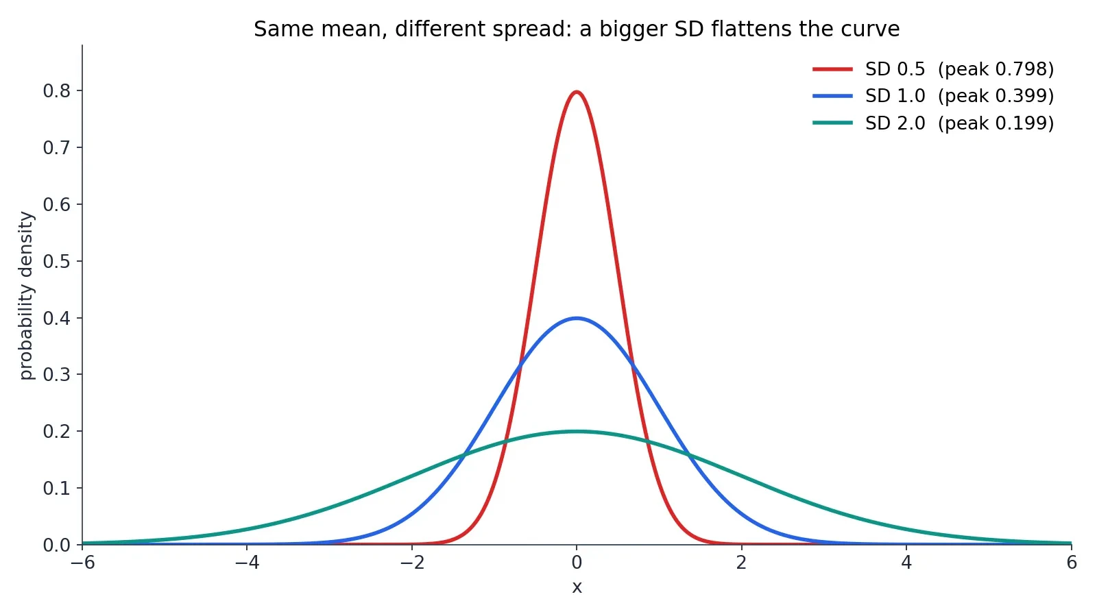
Mu is the mean. It slides the whole curve left and right without changing its shape: raise mu and the hump moves right, lower it and the hump moves left. Sigma is the standard deviation. It stretches the curve wide or squeezes it tall: a bigger sigma spreads the values out, a smaller sigma piles them up near the middle. The constant in front, 1 over the square root of 2 pi times sigma, is there to make the total area exactly 1, so that the curve is a proper probability distribution. The e to a negative square is what makes the bell shape: squaring the distance from the mean makes both sides behave the same way, and the minus sign makes the curve fall as the distance grows. The NIST handbook page on the normal distribution states the same formula and the same roles for mu and sigma, and it is a good place to check them against an authoritative source.
The curve changes direction at exactly one standard deviation either side of the mean. Inside one standard deviation of the mean the curve bends downward; outside it, it bends upward. Those two points, mu minus sigma and mu plus sigma, are called the inflection points, and they are the reason the standard deviation is the natural ruler for this curve: the curve itself marks off one standard deviation on each side of its peak.
The standard normal distribution
There is one master curve from which every other normal curve is made. It has mean 0 and standard deviation 1, and it is called the standard normal distribution. Its peak height is 0.39894, which is 1 over the square root of 2 pi. Every other normal curve is a stretched and shifted copy of this one: stretch it horizontally by sigma, slide it sideways by mu, and squeeze it vertically so the area stays 1, and you have the normal curve with mean mu and standard deviation sigma. That is why the standard normal matters so much. Learn one curve and you have learned them all.
The notation is compact. Writing X follows N(mu, sigma squared) means X is normally distributed with mean mu and variance sigma squared. The variance is sigma squared, the square of the standard deviation, and it appears in the notation because the mathematics works more cleanly with variances than with standard deviations. You will see both forms in textbooks. They say the same thing.
Two numbers describe the whole curve
Here is the fact that makes the normal distribution so powerful. Nothing else is needed. With those two numbers in hand, the curve can be drawn, and the drawn curve answers every "how many" question about the population it describes. No other information is required. Compare that with a distribution like income, where you need to know the shape, the skew, the tail, and a dozen other things before you can say anything useful. The normal distribution is the simplest distribution that describes real data well, and its simplicity is the reason it rules so much of statistics.
That simplicity comes with a warning, and the warning will return throughout this article. The two numbers describe the curve only if the data really is bell-shaped. If the data is skewed, or has two humps, or has a long tail, then the mean and the standard deviation are still numbers you can compute, but the curve they draw will be a lie. Checking the shape comes first. The arithmetic comes second.
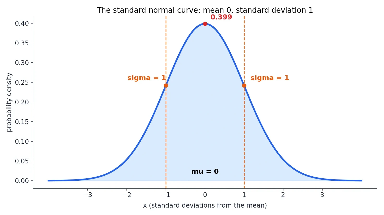
3. Standard Deviation: The Ruler the Bell Curve Is Measured With
The normal distribution is described by two numbers, and the second of them, the standard deviation, does most of the work. The mean tells you where the middle is. The standard deviation tells you how spread out everything is around that middle. Without it, the mean is almost useless: a class with an average height of 170 cm could be full of people between 165 and 175 cm, or it could be a strange mix of very short and very tall people who happen to average out to 170. The standard deviation is what distinguishes those two classes, and it is the ruler the bell curve is measured with.
What standard deviation means
The standard deviation is the square root of the variance, and the variance is the average of the squared deviations from the mean. That definition sounds circular until you unpack it. Take each value, measure how far it sits from the mean, square that distance, average all the squares, and then take the square root to get back to the original units. The result is a typical distance from the mean: a small standard deviation means the values huddle near the mean, and a large standard deviation means they spread out widely. It is denoted by the lowercase Greek letter sigma for a population and by the letter s for a sample.
Think of it as the average surprise. If I tell you a person is 170 cm tall and the standard deviation is 10 cm, then a person of 180 cm is one standard deviation away, mildly surprising but common. A person of 200 cm is three standard deviations away, and that is rare enough to turn heads. The standard deviation turns "tall" from a vague word into a measured distance.
Worked example from scratch
The best way to understand the standard deviation is to compute one by hand. Take a small data set, chosen for clean arithmetic rather than as real measurements: 2, 4, 4, 4, 5, 5, 7, 9. There are 8 values, and they add up to 40, so the mean is 5.0 exactly.
Now measure each value's deviation from the mean: minus 3, minus 1, minus 1, minus 1, 0, 0, plus 2, plus 4. Square each deviation: 9, 1, 1, 1, 0, 0, 4, 16. The squared deviations add up to 32. The population variance is 32 divided by 8, which is 4.0, and the population standard deviation is the square root of 4.0, which is exactly 2.0. That is the answer for this data set, using the population form: the standard deviation is 2.
There is a second form you will meet in textbooks, and the two forms are easy to confuse, so keep them apart. The sample variance divides by n minus 1 instead of n, which is called Bessel's correction. For this data set the sample variance is 32 divided by 7, which is 4.57142857, and the sample standard deviation is 2.138090. The population form answers the question "how spread out are these 8 values?" The sample form answers the question "how spread out is the larger population these 8 values were drawn from?" Use the population form when you have the whole group in front of you, and the sample form when your data is a sample from something bigger. This article uses the population form for the worked example, and says so wherever the distinction matters.
I once spent an afternoon marking exam papers where a student had computed a standard deviation of 2.14 for a data set whose population standard deviation was exactly 2, and had then spent a page apologising for the "error". There was no error. The student had used the sample formula where the question asked for the population formula, and both answers were correct for the question each one was answering. The lesson stayed with me: in statistics, the most common mistake is not bad arithmetic but answering a slightly different question from the one that was asked, and then trusting the answer.
Why square the deviations
Why square the deviations at all? Why not just average the distances from the mean directly? Because the positive and negative deviations cancel each other out. In our data set the deviations add up to zero, exactly, and they always do: the mean is defined as the point where the deviations balance. Averaging the raw deviations would always give zero, which tells you nothing. Squaring stops the cancellation, because a squared number is always positive, whether the original deviation was above or below the mean.
Squaring also punishes big misses more than small ones. A deviation of 4 contributes 16 to the sum, while a deviation of 1 contributes only 1, so a single far-out value counts for far more than several small ones. That is a deliberate choice, and it matches how we think about errors: one measurement that is wildly wrong matters more than several that are slightly off. The square root at the end returns the answer to the original units, centimetres for heights and points for exam marks, so the standard deviation can be compared directly with the values it describes.
A short history of the name
Gauss called the standard deviation the "mean error", which is a good name for what it measures: the typical size of an error. The name we use now, "standard deviation", was first used in writing by Karl Pearson in 1894, after he had used it in his lectures in 1893. Pearson was the great populariser of statistical language, and this is one of the terms that stuck. The idea is older than the name, and the name is younger than the curve, which is a pattern you will see again in the history of this subject: the mathematics arrives first, and the words catch up decades later.
4. Z-Scores: How to Compare Anything to Anything
A height of 185 cm, an IQ of 130, and an exam mark of 85 out of 100. Which of those is the most unusual? The raw numbers cannot answer the question, because they live on different scales with different centres and different spreads. The z-score is the tool that puts them all on one scale. It standardises any value: z equals x minus mu, divided by sigma. It says how many standard deviations a value sits above or below the mean, in units that work for any normal distribution.
A z-score of 0 is exactly average. A z-score of plus 1 is one standard deviation above the mean. A z-score of minus 2 is two standard deviations below the mean. The sign tells you the direction, and the size tells you the rarity. A z-score of 2 on any normal scale means the same thing: the value sits above about 97.7 percent of the population. That is the whole point of standardising. It strips away the units and leaves only the position.
Worked z-scores on the height model
Take the teaching model for heights again: mean 170 cm, standard deviation 10 cm. A height of 150 cm is z equals minus 2. A height of 160 cm is z equals minus 1. A height of 170 cm is z equals 0. A height of 180 cm is z equals plus 1. A height of 190 cm is z equals plus 2. A height of 200 cm is z equals plus 3. Each step of 10 cm is one step of one standard deviation, because the standard deviation is 10 cm.
A height of 185 cm is z equals 1.5, because 185 is 15 cm above the mean and 15 divided by 10 is 1.5. That height is the 93.32nd percentile: it is taller than about 93 in 100 people in this model. A height of 155 cm is z equals minus 1.5, the 6.68th percentile: taller than only about 7 in 100 people. The two heights are mirror images of each other, because the curve is symmetric, and their percentiles add up to 100.
Z-scores on the IQ scale
Now the same arithmetic on the IQ scale, mean 100 and standard deviation 15. An IQ of 130 is z equals 2, exactly as a height of 190 cm was z equals 2. An IQ of 145 is z equals 3, exactly as a height of 200 cm was z equals 3. An IQ of 85 is z equals minus 1, exactly as a height of 160 cm was z equals minus 1. The numbers 130 and 190 look nothing alike, but their z-scores are identical, and so is their rarity: both sit above about 97.7 percent of their populations, and both occur in about 2.28 percent of people.
That is why z-scores matter. They let you say, with a straight face, that an IQ of 130 is exactly as unusual as a height of 190 cm, even though one is measured in points and the other in centimetres. The units fall away and the position remains. A teacher comparing a pupil's maths mark with their English mark, a doctor comparing a patient's blood pressure with their cholesterol, and a factory comparing the length of two different parts are all doing the same thing when they standardise: they are asking how far from average, measured in the natural units of that particular spread.
Percentiles from z-scores
A percentile is just the z-score translated into plain language. The percentile of a value is the share of the population below it, and it comes from the standard normal cumulative probability, written Phi of z. A z-score of 1.5 beats about 93 in 100 people. A z-score of minus 1.5 beats about 7 in 100. A z-score of 2 beats about 97.7 in 100, and a z-score of minus 2 beats about 2.3 in 100.
You do not need a z-table to use this. The numbers in this article are computed directly, and the pattern is what matters: each whole step of one standard deviation moves you much further out into the tail than the last one did. Going from z equals 0 to z equals 1 takes you from the 50th percentile to the 84th, a jump of 34 points. Going from z equals 1 to z equals 2 takes you from the 84th to the 97.7th, a jump of less than 14 points. Going from z equals 2 to z equals 3 takes you from the 97.7th to the 99.87th, a jump of barely 2 points. The tail thins out fast, and that thinning is the bell curve.
A raw number without its z-score can mislead badly, which is a theme our Misleading Statistics article works through in full. A score of 85 sounds ordinary until you learn the mean is 50 and the standard deviation is 10, which makes it three and a half standard deviations above average. A score of 130 sounds impressive until you learn the mean is 125 and the standard deviation is 20, which makes it barely above average. Always ask for the mean and the spread before you judge a number. Without them, the number is a stranger with no context.
5. The 68-95-99.7 Rule: Three Numbers That Answer Almost Every Question
The 68-95-99.7 rule, also called the empirical rule or the three-sigma rule, is the most useful shortcut in all of statistics. It says that for a normal distribution, about 68 percent of values lie within one standard deviation of the mean, about 95 percent within two, and about 99.7 percent within three. Three numbers, and they answer almost every "how many" question you will ever ask about bell-shaped data.
The rounded numbers are enough for most purposes, and they are the ones to memorise. The exact values are 68.27 percent, 95.45 percent, and 99.73 percent, and this article uses the exact values whenever it gives more than the rounded rule. The percentages are rounded theoretical probabilities, not exact guarantees about any particular group of observations. In a real class of 1,000 people you might find 690 between 160 and 180 cm instead of 683, or 670. The rule describes the curve, and real groups wobble around it.
The height model, worked end to end
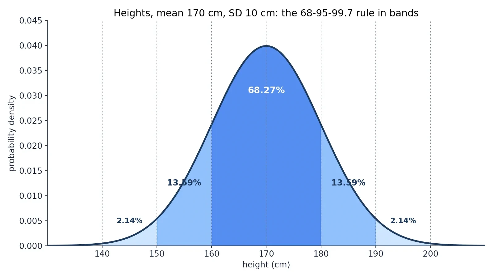
Take the teaching model again: mean 170 cm, standard deviation 10 cm. Between 160 and 180 cm, one standard deviation either side of the mean, sit 68.27 percent of people: about 683 of 1,000. Between 150 and 190 cm, two standard deviations either side, sit 95.45 percent: about 955 of 1,000. Between 140 and 200 cm, three standard deviations either side, sit 99.73 percent: about 997 of 1,000. Only about 3 people in 1,000 fall outside the range from 140 to 200 cm.
The tails tell the same story from the other side. Taller than 190 cm: 2.28 percent, about 23 in 1,000. Shorter than 150 cm: the same 2.28 percent, about 23 in 1,000, because the curve is symmetric. Taller than 200 cm: 0.13 percent, about 1 in 741. The same arithmetic as the opening of this article, and now you can see where every number came from.
| Range (height model) | Exact share | Rounded share | People in 1,000 |
|---|---|---|---|
| Within 1 SD: 160 to 180 cm | 68.27 percent | about 68 percent | about 683 |
| Within 2 SD: 150 to 190 cm | 95.45 percent | about 95 percent | about 955 |
| Within 3 SD: 140 to 200 cm | 99.73 percent | about 99.7 percent | about 997 |
| Taller than 190 cm (above 2 SD) | 2.28 percent | about 2.3 percent | about 23 |
| Taller than 200 cm (above 3 SD) | 0.13 percent | about 0.1 percent | about 1 |
The bands between the lines
The rule hides a finer structure that is worth knowing. The 68.27 percent within one standard deviation splits into two equal halves: 34.13 percent between the mean and one standard deviation above it, and 34.13 percent between the mean and one standard deviation below it. The band between one and two standard deviations holds 13.59 percent on each side. The band between two and three standard deviations holds 2.14 percent on each side. Add them up on one side: 34.13 plus 13.59 plus 2.14 equals 49.86 percent, and the remaining 0.14 percent lies beyond three standard deviations. Both sides together give the familiar 99.73 percent.
This is the arithmetic behind the everyday phrase "about two-thirds are within one standard deviation". It also explains why the curve feels so concentrated: half the population sits within two-thirds of a standard deviation of the mean, and almost everything sits within three. The tails exist, but they are thin, and they get thinner fast.
Beyond 3 SD, and the 1.96 shortcut
About 1 value in 370 lies beyond three standard deviations on either side combined. That is a useful number to carry around: in a school of 370 pupils, you expect about one pupil to be more than three standard deviations from the mean on any given bell-shaped measurement. It is not a sign that something is wrong with that pupil. It is the curve doing what the curve does.
There is one more number worth knowing, because it runs half of modern statistics. Within 1.96 standard deviations sit 95.000421 percent of values, which is why the 95 percent confidence interval is built from 1.96 standard deviations either side of an estimate. The rounded rule says 2 standard deviations for 95 percent, and 1.96 is the exact version of that shortcut. Within 2.58 standard deviations sit 99.01 percent of values, which is the basis of the 99 percent confidence interval. The rule and the confidence interval are the same mathematics, used for different jobs.
The Chebyshev safety net
What if the data is not bell-shaped at all? Then the 68-95-99.7 rule does not apply, and using it anyway is one of the most common mistakes in statistics. But you are not left with nothing. Chebyshev's inequality guarantees that for any distribution with a finite mean and variance, at least 75 percent of values lie within two standard deviations and at least 88.89 percent within three. Those guarantees are much weaker than the normal curve's 95.45 and 99.73 percent, and that is the price of knowing nothing about the shape. The normal curve beats the guarantee precisely because it assumes the bell shape, and that assumption must be checked before the rule is used. This is the bridge to the later section on where the bell curve fails. Use the rule only after you have looked at the shape.
6. The Central Limit Theorem: Why So Much of the World Is Bell-Shaped
Here is the deepest fact in this article, and the reason the bell curve shows up in so many places that it seems to rule the world. The central limit theorem says that averages of many independent observations are approximately normal, whatever the original observations look like. Add up many small independent effects and the total is bell-shaped, even if none of the individual effects is bell-shaped at all. The bell curve is not one shape among many. It is the shape that sums take.
Think about a measurement error. A single measurement of a star's position is disturbed by a dozen tiny things: a tremor in the telescope, a flicker in the air, a rounding in the reading, a wobble in the clock. None of those disturbances is bell-shaped on its own. But their sum is, because the sum of many small independent effects is always approximately normal. That is why Gauss found the bell curve in astronomy, and why it still turns up in every laboratory that repeats a measurement.
The theorem in plain English
The classical form of the theorem, called the Lindeberg-Levy central limit theorem, goes like this. Take independent observations from the same distribution, each with mean mu and finite positive variance sigma squared. Then for large n, the sample mean is approximately normal with mean mu and variance sigma squared over n. Equivalently, the sum is approximately normal with mean n times mu and variance n times sigma squared. The bigger n gets, the better the approximation, and the error shrinks like 1 over the square root of n, which is the Berry-Esseen bound stated in words.
The standard error of a sample mean is sigma over the square root of n, and that single formula explains why averages of larger samples vary less. Double the sample size and the standard error falls by a factor of about 1.41, not by half. Quadruple it and the standard error halves. Pollsters, quality controllers, and medical researchers all live by this arithmetic: precision grows with the square root of the sample size, never faster.
The conditions, in plain terms
The theorem has conditions, and they matter. The observations must be independent, so that one does not push the next one around. The variance must be finite, so that no single wild value can dominate the total. And no single observation is allowed to dominate the sum, which is the Lindeberg condition: for every positive margin, the contribution to the total variance from terms beyond that margin must shrink to zero as n grows. There is a stronger, easier-to-check condition called the Lyapunov condition, which says that if the sum of the third absolute moments grows slowly enough relative to the total variance, the theorem holds. If Lyapunov holds, Lindeberg holds; the reverse is not true.
The finiteness of the variance is essential, and there is a famous counterexample that shows why. The average of independent Cauchy random variables has the same Cauchy distribution for every n. It does not concentrate at all, no matter how many you average, because the Cauchy distribution has no finite variance and its wild values keep dominating the sum. The theorem fails there, and it fails for exactly the reason the conditions warn about: one observation can still dominate the total.
What the theorem does NOT say
The most common misunderstanding of the central limit theorem is also the most damaging. It does not say that data become more normal as you collect more of them. It is about sums and averages, not about individual observations. A skewed population stays skewed no matter how large the sample. Only the distribution of its sample means becomes bell-shaped. Gathering more height measurements leaves the shape of the height distribution exactly as it was. Collecting more incomes does not make income bell-shaped. The theorem describes what happens when you average, not what happens when you measure.
Dice, the five-minute demonstration
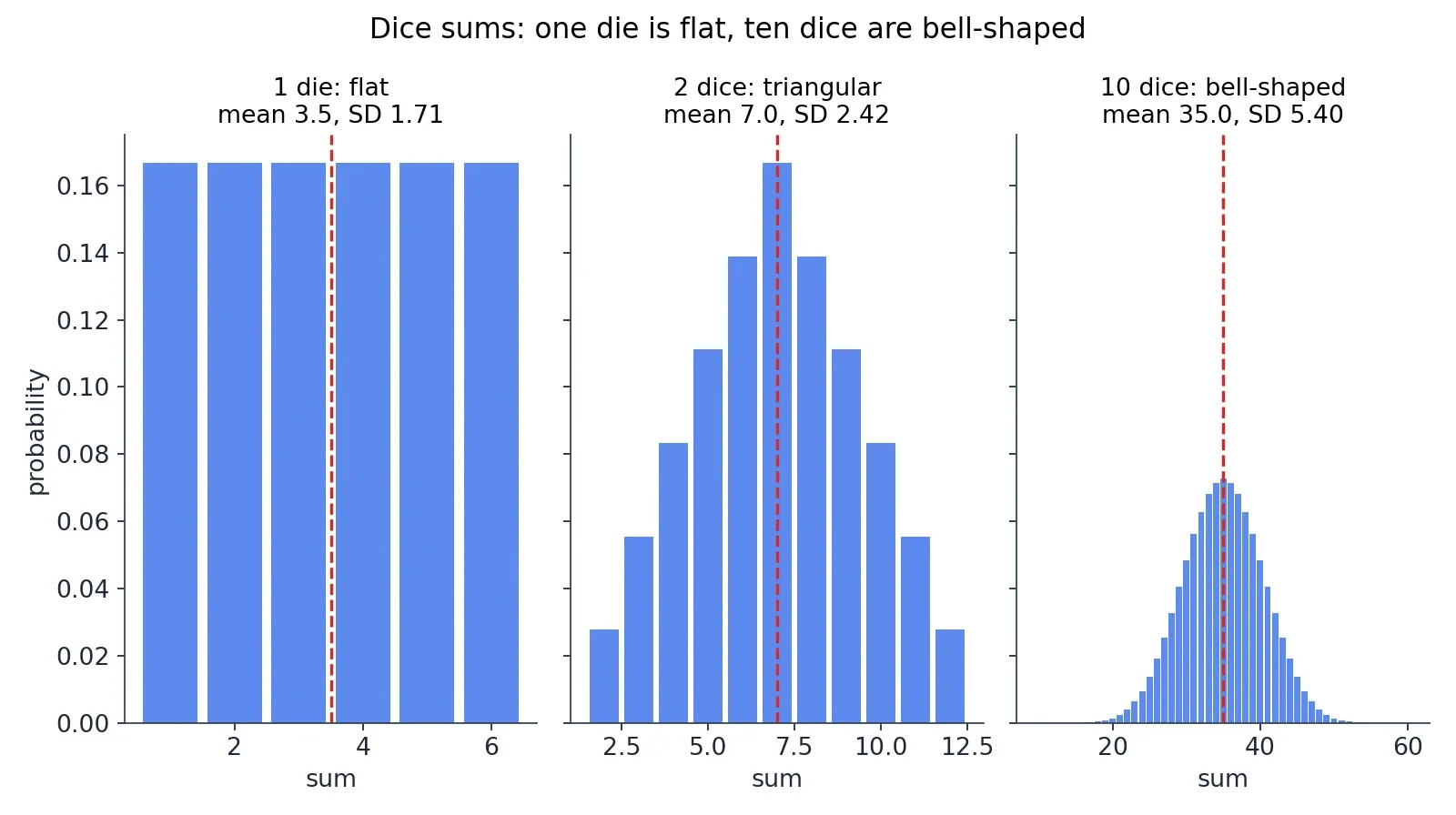
The fastest way to see the theorem working is with dice. One die is flat: each face from 1 to 6 comes up 1 time in 6, and the distribution is a row of six equal bars. Two dice make a triangle: the sum 7 is the most likely, the sums 2 and 12 are the least likely, and the probabilities rise and fall in straight lines. Ten dice make a bell shape: the sum has mean 35 and standard deviation 5.40, and the distribution is already visibly curved, with the middle sums far more likely than the extremes. Nothing about a single die is bell-shaped. The bell appears only when you add them up, and ten is already enough to see it clearly.
I have run this demonstration in a classroom with a cup of dice and a tally sheet, and the moment the ten-dice histogram starts curving is the moment the room understands the theorem. The students expect the curve to need some special ingredient, some hidden bell hidden inside each die. There is none. The bell is what addition does. The area under the curve is an integral, and the way the area accumulates as you add more dice is the same calculus our Calculus article builds from first principles.
7. Three Centuries of One Curve: De Moivre, Laplace, Gauss, Quetelet, Galton, Pearson
The bell curve is nearly 300 years old, and its history is a story of the same idea being found again and again, each time in a new disguise: first as a gambling problem, then as a theorem about averages, then as the law of errors, then as a description of people, and finally as a machine made of pegs and beads. The names attached to it are the great names of probability, and each of them added a piece that the others had missed.
De Moivre, 1733
The curve first appeared as an answer to a gambling problem. Abraham de Moivre, a French-born mathematician living in London, wanted to approximate binomial probabilities for many coin tosses. Computing the exact probability of, say, 60 heads in 100 tosses by hand was a long slog through factorials, and de Moivre found a shortcut: as the number of tosses grows, the binomial probabilities trace out a smooth bell-shaped curve. He wrote the result in a privately circulated Latin pamphlet in November 1733, "Approximatio ad Summam Terminorum Binomii (a plus b) to the power n in Seriem expansi", of which only two copies are known to survive. His own English translation, with additions, appeared in the second edition of The Doctrine of Chances in 1738, on pages 235 to 243.
De Moivre's paper gave the first occurrence of the normal probability integral, and he appears to have perceived, without naming it, the parameter we now call the standard deviation. He used Stirling's formula, which he had found before Stirling, to derive the curve. The Doctrine of Chances itself appeared in editions in 1718, 1738 and 1756, and it was the standard textbook of probability for most of the eighteenth century. The MacTutor biography of de Moivre tells this story in full, and it is the best place to check the dates. Note the date carefully: November 1733, with no specific day, because the two surviving accounts disagree about whether the pamphlet was dated the 12th or the 13th, and the month is all that both agree on.
Laplace, 1810-1812
Pierre-Simon Laplace took de Moivre's special case and turned it into a general theorem. In two papers in 1810 and 1811 he proved the first general central limit theorem, developing the characteristic function as a tool for large-sample theory. His most general statement is in Chapter 3 of Book II of the Theorie analytique des probabilites, published in 1812: when the number of independent observations increases, the distribution of their mean tends toward a Gaussian form regardless of the distribution of the individual observations. That sentence is the central limit theorem as we know it, and it is the reason the bell curve is everywhere.
The de Moivre-Laplace theorem is the first version of the central limit theorem: the special case of a fair coin was de Moivre's, and the general case was Laplace's. Laplace had used the normal curve to describe the distribution of errors from 1783, long before the general theorem, which is a reminder that in mathematics the tool often arrives before the proof that justifies it. The full rigorous proof had to wait for Lyapunov in 1901 and 1902, and the theorem was only stated in its modern form in the 1920s. A theorem can be true and useful for a century before anyone proves it properly.
Gauss and Adrain, 1808-1809
The curve's next home was astronomy. Carl Friedrich Gauss published Theoria motus corporum coelestium in 1809, in which he derived the normal distribution from the method of least squares: if measurement errors follow the bell curve, then least squares gives the most probable answer. That is why the distribution is also called the Gaussian distribution. Gauss had a rival for the idea, and the rival got there first. Robert Adrain independently derived the normal error law in 1808, a year before Gauss, though his work was published in a journal few people read and was largely forgotten until historians recovered it.
Adrien-Marie Legendre had published the method of least squares in 1805, without a probabilistic justification. Gauss supplied the justification in 1809 and said he had used the method since 1795, a priority claim that is still disputed and should not be presented as settled fact. Gauss later gave a second, stronger justification of least squares, free of the normality assumption, in the Theoria combinationis of 1823, which is the result now called the Gauss-Markov theorem. The first justification made the bell curve famous. The second showed that least squares could survive without it.
Quetelet, 1835-1846
Adolphe Quetelet, a Belgian mathematician and astronomer, was the first to apply the normal distribution to human characteristics, and the first to use the normal curve for anything other than a law of errors. He introduced the "average man", l'homme moyen, in Sur l'homme et le developpement de ses facultes, published in 1835 and translated into English in 1842 as A Treatise on Man. His idea was that human measurements, heights and chest sizes and weights, scatter around an average in the same bell shape as astronomical errors, and that the average itself was the true human being.
In 1846 Quetelet published the chest measurements of 5,738 Scottish soldiers and showed they formed a bell curve around roughly 40 inches, an average just over 39 and three-quarter inches. He did not measure the soldiers himself: the figures came from an Edinburgh medical journal of 1817. Later scholars found errors in his arithmetic when adding up the measurements, which is a useful reminder that even a great idea can rest on shaky counting. Around 1832 Quetelet also observed that adult weight is roughly proportional to the square of height, and that ratio, weight in kilograms divided by height in metres squared, was named the body mass index in 1972 by Ancel Keys.
Quetelet's interpretation needs to be read critically, and modern readers should. He treated the individual person as synonymous with error and the average person as the true human being: the average as an ideal, not just a summary. That is a strange and dangerous idea when it leaves mathematics and enters thinking about people, because no real person is average in every way at once, and treating the average as the ideal turns ordinary human variation into a defect. The statistics was sound. The philosophy was not.
Galton, 1873-1889
Francis Galton took Quetelet's idea and ran with it, and he also built the machine that demonstrates the central limit theorem better than any equation. He invented the Galton board, the quincunx or bean machine, and first demonstrated it at a Royal Institution discourse on 27 February 1874. The board was manufactured by Tisley and Spiller in 1873, and it had 19 rows of pegs and 10 bead bins. Galton used the phrase "deviated normally" in 1877, and began using "normal" systematically in the 1880s. Chapter 5 of his Natural Inheritance, published in 1889, is entitled "Normal Variability". He also developed regression toward the mean, which he called "reversion to mediocrity", and the bivariate normal distribution.
Galton was also a founder of eugenics, and his work on human measurement was bound up with that programme. That fact belongs in any honest account of him, and it is a reason to read his work with care rather than with admiration alone. The mathematics he built is sound and beautiful. The uses he imagined for it were not.
Pearson, 1893-1894
Karl Pearson popularised the name "normal curve", and the story of how he did it is a lesson in how scientific language spreads. In "Contributions to the Mathematical Theory of Evolution", published in the Philosophical Transactions of the Royal Society of London A, volume 185, in 1894, he wrote on page 72 that a frequency curve which could practically be represented by the error curve would for the rest of the paper be termed a normal curve. He did not invent the term. The American C. S. Peirce had used it in 1873, and Galton and Wilhelm Lexis had both used it in the 1870s, apparently independently. But Pearson used it consistently and exclusively in his epoch-making publications, and that consistency is what led to its adoption throughout the statistical community.
Pearson later implied that he had introduced the term himself, writing in Biometrika in 1920 that many years earlier he had called the Laplace-Gaussian curve the normal curve. He also came to regret the name, because it made every other distribution sound abnormal. The regret was justified, and it is still the best argument against the name: "normal" suggests that everything else is a deviation from the proper order of things, and that is simply not true of distributions.
The name settles
The phrase "normal distribution" appears in print in Pearson's 1897 paper on skew variation, and by the early twentieth century the name had settled for good. The curve had been the law of errors, the Gaussian law, Laplace's second law, and the error curve before it became the normal distribution, and the name it kept was the one Pearson pushed hardest, not the one anyone invented first. Stahl's history of the curve, "The Evolution of the Normal Distribution", published in Mathematics Magazine in 2006, won the Mathematical Association of America Writing Award in 2007, and it remains the best single account of this long and tangled naming story.
8. The Galton Board: Watching the Bell Curve Build Itself
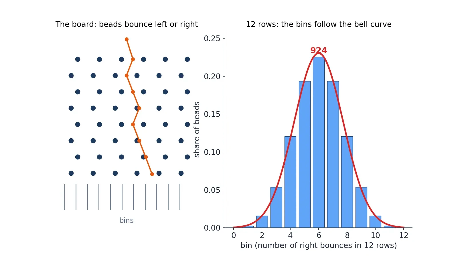
The Galton board is the central limit theorem made of wood and steel, and it is the most convincing demonstration in this article because you can watch it happen. A vertical board is studded with interleaved rows of pegs. Beads drop from the top, bounce left or right with a 50-50 chance at each peg, and collect in bins at the bottom. The column heights in the bins approximate a bell curve, and they do it without any mathematics at all: the machine builds the curve out of pure chance.
I once watched a museum demonstrator run a Galton board for a school group, and the children's reaction was the same as the audience's reaction to the height numbers: disbelief, then delight. They expected the beads to pile up evenly, or randomly, or in a heap under the drop point. Instead the middle bins filled up first and the outer bins stayed nearly empty, and the outline of the columns curved smoothly down on both sides. One child asked who had told the beads where to go. Nobody had. The bell curve is what happens when a thousand small random choices add up.
Why the bins are binomial
A bead that bounces right k times in n rows lands in bin k, so the bin counts follow the binomial distribution. With 12 rows, the middle bin, bin 6, holds 924 of the 4,096 possible paths, which is 22.56 percent of all beads. Each end bin holds just 1 of the 4,096 paths, which is 0.024 percent. The mean bin is 6, the variance is 3, and the standard deviation is 1.73 bins. With 10 rows, the middle bin holds 252 of 1,024 balls, which is 24.61 percent. These numbers are exact, computed from the binomial coefficients, and they are the reason the middle bins fill first: there are simply far more paths that end in the middle than paths that end at the edges.
Why the bins are normal
The de Moivre-Laplace theorem says that with many rows and many balls, the binomial bin counts approximate the normal curve. Each bounce is a tiny independent nudge, left or right, and the total is the sum of many nudges. The central limit theorem does the rest. The dice in the previous section made the same point with numbers. The Galton board makes it with beads you can see and hear, and the lesson is the same: the bell curve is what sums look like.
The second lesson of the board
Galton built the board to show a second idea as well: regression to the mean. Beads that bounce far to one side on the upper rows tend to come back toward the middle on the lower rows, because each new bounce is a fresh 50-50 chance that does not remember the ones before it. Extremes tend to come back toward the middle, not because anything pushes them there, but because the middle is where most of the paths lead. That idea, that an extreme measurement is likely to be followed by a less extreme one, is one of the most useful and most misunderstood ideas in statistics, and the board shows it in a form a child can grasp.
9. The Bell Curve at Work: Heights, IQ Scores, Exams and Measurements
The curve earns its reputation in the working world, where it turns up in four places that matter to almost everyone: heights, IQ scores, exam results, and measurement error. Each of them teaches a different lesson about the curve, and together they show both its power and its limits.
Heights
The teaching model for this article uses mean 170 cm and standard deviation 10 cm, and the numbers it produces are the ones you have already met: about 683 of 1,000 people between 160 and 180 cm, about 23 taller than 190 cm, about 1 taller than 200 cm. Real textbook values for United States adults are a little different: men average 70 inches with a standard deviation of 3 inches, and women average 64.5 inches with a standard deviation of 2.5 inches. Use one set consistently and do not mix sets in one paragraph, because the two sets describe different populations and their numbers will not agree.
Height is approximately normal only within a single homogeneous group. Mix men and women together, or mix populations with very different average heights, and the combined distribution is no longer a single bell curve. The Netherlands, where the average man is about 183.8 cm, mixed with a population where the average man is 170 cm, would give two humps, not one. The 68-95-99.7 rule applies to the single group, never to the mixture. Always check what population your numbers describe before you apply the rule.
IQ scores
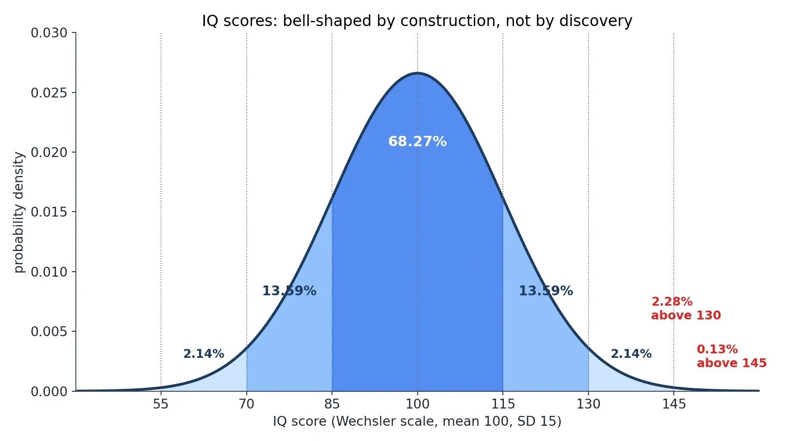
IQ scores are the most misunderstood application of the bell curve in this article, and the misunderstanding matters, so read this part carefully. IQ scores are normally distributed by construction, not by discovery. Test makers rescale raw scores so that the norming sample has mean exactly 100 and standard deviation exactly 15. The bell curve is the output of that standardisation, not its input. The scores are bell-shaped because the test makers made them bell-shaped.
The deviation IQ was formalised by David Wechsler in 1939, replacing the older mental-age ratio method. The mean of 100 was kept for continuity, and the standard deviation of 15 was chosen because it matched empirical data and gave round cutoffs at one, two and three standard deviations. About 68 percent of people score between 85 and 115, about 95 percent between 70 and 130, and roughly 99.7 percent between 55 and 145, as the Psychologic guide to the IQ bell curve sets out in full. Those are the same 68-95-99.7 numbers you already know, wearing different clothes.
How the norming works is the key to the whole story. Test makers give the test to a large normative sample, typically 2,000 to 4,000 people stratified by age, sex, education and ethnicity, rank the raw scores, convert the ranks to z-scores through the normal distribution, and rescale to mean 100 and standard deviation 15. The WAIS-IV standardisation sample was 2,200 adults. The WAIS-5, the newest edition of the Wechsler Adult Intelligence Scale, was published in 2024 with updated norms, which means the norms are remade every generation and "average" is always relative to the current norming sample. A score from an older edition is a rank against a different group of people.
The numbers follow the same arithmetic as the height example. Above IQ 130, which is z equals 2, sit 2.28 percent of people, about 1 in 44. Above IQ 145, which is z equals 3, sit 0.13 percent, about 1 in 741. Below IQ 70, which is z equals minus 2, sit 2.28 percent, about 1 in 44. Above IQ 160, which is z equals 4, sit 0.0032 percent, about 1 in 31,574. In a group of 1,000 people, about 23 score above 130, about 1 scores above 145, about 23 score below 70, and about 683 score between 85 and 115. The thresholds are exact: the top 1 percent starts at IQ 134.90, the top 0.1 percent at 146.35, and the top 2 percent, the usual Mensa admission level, at IQ 130.81, so the commonly quoted 130 is a rounded version of 130.81.
Different tests have used different standard deviations over the years, which is another reason to read the fine print. Wechsler and the modern Stanford-Binet 5 use a standard deviation of 15. The older Stanford-Binet used 16, and the Cattell Culture Fair test used 24. Every IQ number in this article is on the Wechsler scale, standard deviation 15, and every IQ number you meet anywhere else should come with its scale attached. An IQ of 130 on one scale is not the same rarity as an IQ of 130 on another.
| IQ score | Z-score | Percentile | Share above | About 1 in |
|---|---|---|---|---|
| 70 | minus 2 | 2.28th | 97.72 percent | 44 (below) |
| 85 | minus 1 | 15.87th | 84.13 percent | 6 (below) |
| 100 | 0 | 50th | 50.00 percent | 2 |
| 115 | plus 1 | 84.13th | 15.87 percent | 6 |
| 130 | plus 2 | 97.72nd | 2.28 percent | 44 |
| 145 | plus 3 | 99.87th | 0.13 percent | 741 |
I once watched a parent wave a child's test report in a meeting and announce that the child was "in the top 2 percent", as if that number described something fixed in nature. The number described a rank against a norming sample, built by people who chose the mean and the standard deviation in advance. The child had done well on a test, and that was real. But the bell curve around the score was not a discovery about the child's mind. It was a decision by the test makers, and knowing that changes how seriously you should take the third decimal place.
Test scores and test results both need a base rate before they mean anything, and our Bayes article is the full story of that idea. An IQ score is a measurement with a chosen scale. A medical test result is a measurement with a chosen threshold. Both are only as meaningful as the population they were standardised against.
SAT scores
The SAT is the exam-driven version of the same story, and it comes with a warning. The textbook model treats combined SAT scores of college-bound seniors as normal with mean 1050 and standard deviation 150. On that model the middle 68 percent score between 900 and 1200, the chance of scoring between 900 and 1500 is 84.00 percent, the chance of scoring above 1350 is 2.28 percent, and the chance of scoring above 1500 is 0.13 percent. The 97.5th percentile is 1344, which textbooks often round to about 1350.
Two corrections matter here, and both are the kind of small error that spreads through textbooks unnoticed. A widely copied review gives 83.85 percent for the chance of scoring between 900 and 1500. That figure is wrong. The correct value, recomputed from the model, is 84.00 percent. And the 97.5th percentile is 1344, not 1350, though "about 1350" is a fair rounding. Small errors, but they are the reason this article recomputes every number instead of copying it.
The bigger warning is that real SAT scores are only approximately normal. Real scores come in steps of 10, they are capped at 400 and 1600, and they come from a self-selected group of test takers, so a normal-curve calculation can land several percentile points away from the College Board's published table. Use the SAT numbers as a teaching model, and never compute a real person's percentile from the normal curve as if it were the official table. The model teaches the method. The table gives the answer.
Measurement error and quality control
Measurement error was the original home of the normal curve, and it is still the cleanest example of why the curve works. Repeated measurements of the same quantity scatter around the true value in a bell shape, because each measurement error is the sum of many tiny independent disturbances. That was Gauss's insight in astronomy, and it is the same logic that covers manufacturing, where parts machined to a target size vary in a bell shape, and laboratory assays, where repeated readings of the same sample scatter around the true value. A process centred on target with small random errors produces bell-shaped variation, and quality control is built on that fact.
Different fields demand different levels of proof before they call something a discovery, and the difference is measured in standard deviations. In particle physics, a discovery conventionally requires a five-sigma effect, which is 99.99994 percent confidence. In the social sciences, a two-sigma effect, 95 percent, is often treated as worth closer examination. The numbers are the same curve. The standards are different because the costs of being wrong are different.
The statistical toolkit that runs on the curve
The normal distribution underlies the most common statistical tools in use today: confidence intervals for means, z-tests and t-tests, control charts with three-sigma limits, and regression. The regression point needs to be stated precisely, because it is often stated wrongly: in regression it is the residuals, the errors left over after the model has done its work, that are assumed normal, not the outcome variable itself. The outcome can be as skewed as you like, provided the errors around the fitted line are bell-shaped. Getting that distinction right is the difference between a model that works and a model that quietly lies.
10. Normal Approximations: When the Bell Curve Stands In for Something Else
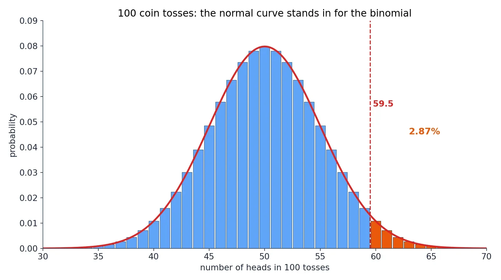
The bell curve is useful even when the data is not normal at all, because it can stand in for other distributions when the numbers get large. The most important of these stand-ins is the normal approximation to the binomial, which is the de Moivre-Laplace theorem in working clothes: a binomial distribution with parameters n and p is approximately normal with mean n times p and variance n times p times 1 minus p, when n is large. De Moivre found it for coin tosses in 1733. Laplace generalised it. It is still the fastest way to answer "how likely is this many heads?"
There is a rule of thumb for when the approximation is safe: n times p and n times 1 minus p should both be at least 5, though some textbooks say 10. That is a textbook rule of thumb, not a theorem, and it should be labelled as such. It says, in plain language, that you need enough expected successes and enough expected failures for the bell shape to have room to form. A binomial with n equal to 5 is a row of six spikes, not a bell. A binomial with n equal to 100 is a bell with a slight staircase texture.
Worked example A: 100 fair coin tosses
Toss a fair coin 100 times. The mean number of heads is 50, and the standard deviation is 5. What is the chance of 60 or more heads? The exact answer is 2.84 percent. The normal approximation with the continuity correction gives 2.87 percent: z equals 59.5 minus 50, divided by 5, which is 1.9, and the tail beyond z equals 1.9 is 0.0287. Without the continuity correction, z equals 2.0 gives 2.28 percent, which is noticeably worse. The lesson is the whole point of this section: use 59.5, not 60, because the bar for "60 heads" in the histogram runs from 59.5 to 60.5, and the normal curve needs to start at the left edge of that bar.
Worked example B: 200 trials, probability 0.3
Take n equal to 200 and p equal to 0.3. The mean is 60 and the standard deviation is 6.4807. The exact chance of 50 or fewer successes is 6.95 percent. The continuity-corrected approximation gives 7.13 percent: z equals 50.5 minus 60, divided by 6.4807, which is minus 1.4659. The approximation is a little high, and that is honest: approximations have errors, and the error here is about two-tenths of a percentage point on a 7 percent answer. Good enough for a quick judgement, not good enough for a published result.
Worked example C: the Poisson approximation
The same trick works for the Poisson distribution, which describes counts of rare events. Take lambda equal to 16. The exact chance of 10 or fewer events is 7.74 percent. The normal approximation with mean 16 and standard deviation 4, with the continuity correction, gives 8.46 percent: z equals 10.5 minus 16, divided by 4, which is minus 1.375. The approximation is rougher here, because lambda equal to 16 is only moderately large, and the Poisson distribution at lambda 16 is still visibly skewed. The approximation improves as lambda grows, and that is worth saying plainly: the bell curve stands in well for a nearly symmetric distribution, and less well for a skewed one.
The extra check
One more comparison shows how good the approximation can be when the conditions are right. The chance of between 45 and 55 heads in 100 tosses is 0.728747 exactly, and the normal approximation with the continuity correction gives 0.728668. The two agree to three decimal places. When the interval sits in the fat middle of the distribution, where the curve is smooth and the bars are tall, the approximation is superb. When the interval sits in the thin tail, where the curve is steep and the bars are short, the approximation is rougher. That pattern, good in the middle and rougher in the tails, is the signature of every approximation in this article.
11. Where the Bell Curve Fails: Income, City Sizes and the Data That Refuse to Be Normal
Everything so far has been a celebration of the bell curve, and the celebration is deserved. But the curve fails often enough, and badly enough, that the failures deserve their own section. A tool used on the wrong shape does not give a slightly wrong answer. It gives a confidently wrong answer, and confidence is the dangerous part.
Income
Income is not normally distributed. Personal income is right-skewed: most people cluster at low-to-moderate incomes, a long tail stretches to very high incomes, and the mean systematically exceeds the median, so symmetric Gaussian distributions are inapplicable. The 68-95-99.7 rule applied to income would tell you that almost nobody earns more than three standard deviations above the mean, and it would be wrong by orders of magnitude, because the tail of the income distribution is fat with people the bell curve says should barely exist.
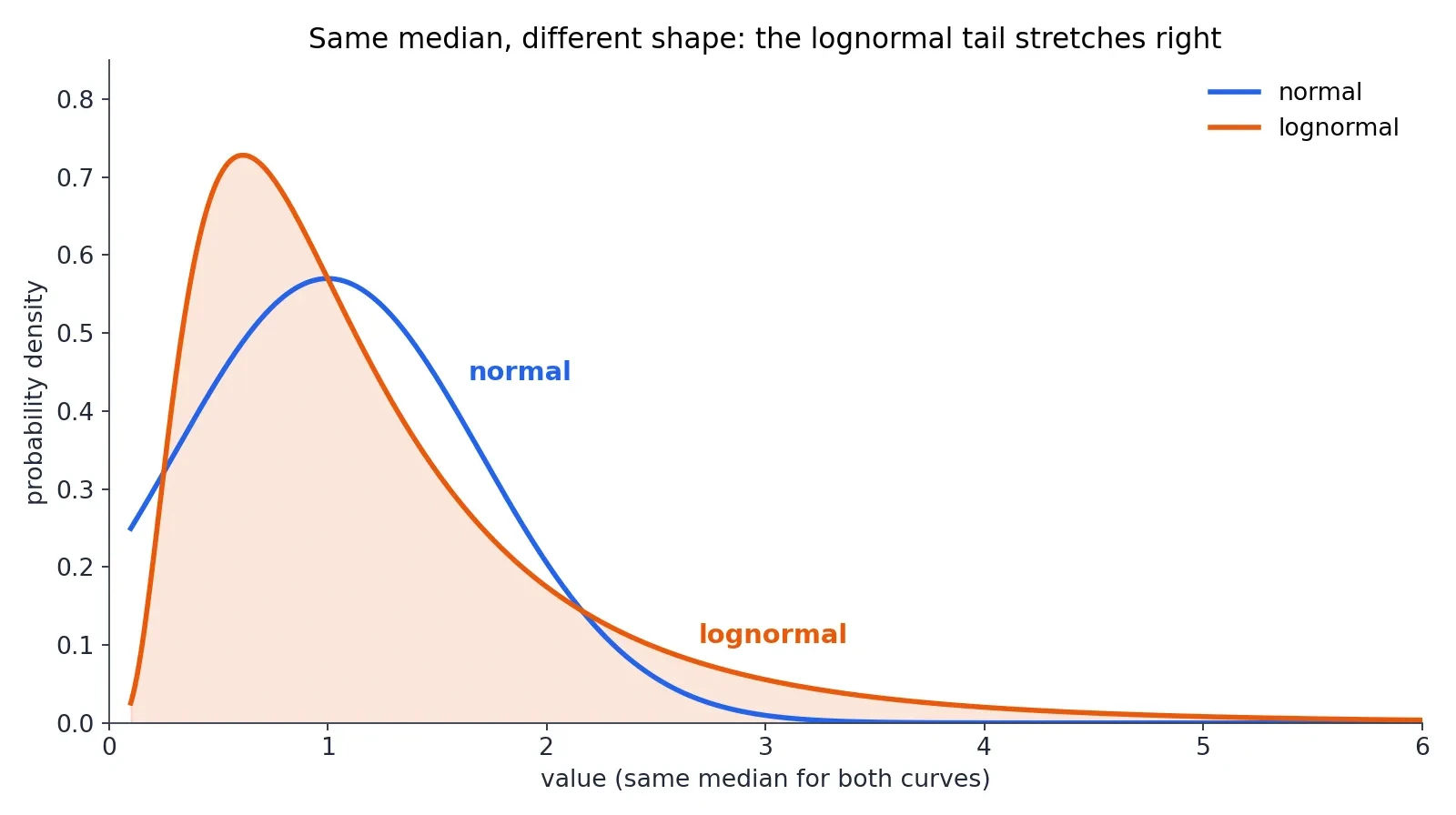
The standard model of income is lognormal for the middle range with a Pareto power-law tail for the richest few percent: lognormal in the middle, following Gibrat's work of 1931, and Pareto in the upper tail, following Pareto's work of 1897. For 1935-36 United States data, the top 1 percent followed a Pareto distribution with alpha equal to 1.63, and the rest followed a lognormal. In modern economies the Pareto index alpha typically ranges between 1.5 and 2.5. The exact value moves around, but the shape does not: a hump in the middle and a long tail on the right.
What lognormal means
A variable is lognormally distributed when its logarithm is normally distributed. Lognormal variables are always positive and right-skewed, and income, city sizes and stock prices are the classic examples. The idea is simple once you see it: take the logarithm of incomes and the bell curve comes back, and our Logarithms article is the full story of why logarithms straighten skewed data. The logarithm compresses the long right tail and stretches the bunched-up left side, and the skewed curve becomes symmetric. That is what a lognormal distribution is, and it is the direct bridge between this article and the article on logarithms.
City sizes
City sizes refuse the bell curve in the same way. National and regional city size distributions are lognormally distributed through the majority of cities and only approach power functions, Zipf's law, for the largest cities in the tail. Zipf observed in 1949 that a city's population is roughly proportional to the inverse of its rank: the second city is about half the size of the first, the third about a third, and so on. The literature disagrees on the details, and one study of United States cities concludes that the entire distribution is not lognormal and that Zipf's law does not hold generally, with a power-law tail that is robust. The honest summary is the lognormal-plus-Pareto-tail picture, with the debate noted rather than settled.
The newest evidence points the same way. A November 2026 study of United States employer firms from 1978 to 2023 finds that a lognormal is preferred over a Pareto in all 46 years, yet underpredicts the number of firms with 10,000 employees or more by a factor of 21. The distribution is a mixture whose tail alone is consistent with a power law. The body is lognormal. The tail is Pareto. Neither alone tells the story.
Psychological data
Psychological and mental-health data often violate normality, and the violation is not a technicality. Stress, anxiety and substance use frequently show skewed, zero-inflated or asymmetric distributions, making parametric methods inappropriate and potentially misleading. A 2025 paper in PLOS Mental Health argues exactly this: psychological data often violate normality assumptions through skewness, kurtosis, ordinal scaling and outliers, the violations increase the risk of both kinds of statistical error and bias effect estimates, and the paper advocates assumption-light methods such as bootstrapping and Monte Carlo simulation. When the data is not bell-shaped, the honest move is to use a method that makes no shape assumption at all.
Other shapes in one line each
Bimodal data has two humps, for example when two different populations are mixed together. Uniform data gives every value the same probability, like a fair die. Exponential data describes waiting times, where short waits are common and long waits are rare. Heavy-tailed financial returns produce extreme events far more often than the bell curve predicts, which is why market crashes keep surprising people who priced risk with a normal model. And the mixture warning covers them all: combining two different normal distributions does not give a normal distribution. Always check the shape before applying the 68-95-99.7 rule.
12. Eight Mistakes to Never Make About the Bell Curve
The curve is simple, and its simplicity invites mistakes. Here are the eight that matter most, each with the correction and the one number that proves it.
- "Normal means most things are normal, and everything else is abnormal." False. "Normal" here is a technical term for the shape that sums of small independent effects take, not a judgement that a value is healthy, correct or typical. A non-normal distribution is not a diseased one. Pearson himself regretted the name for this reason, and his own words are worth quoting exactly as he wrote them in 1894.
"A frequency-curve, which for practical purposes, can be represented by the error curve, will for the remainder of this paper be termed a normal curve." — Karl Pearson, 1894
- "Everything in nature is bell-shaped." False. Heights and measurement errors are approximately bell-shaped. Income, city sizes, waiting times and psychological symptom scores are not. The central limit theorem explains averages, not every variable.
- "The 68-95-99.7 rule works on any data set." False. It is a property of the normal model. For any distribution at all, Chebyshev only guarantees 75 percent within two standard deviations and 88.89 percent within three. Check the shape first. We cover how averages mislead in our Misleading Statistics article; the bell curve is the tool that keeps them honest.
- "A bigger sample makes the data more normal." False. The central limit theorem is about the distribution of sample means, not about the raw data. Collecting more height measurements does not change the shape of the height distribution.
- "IQ 100 is the average because intelligence is naturally bell-shaped." False, or at least backwards: IQ scores are bell-shaped because test makers rescale them to be bell-shaped. The bell curve is imposed, not discovered.
- "Being 3 standard deviations out means something is wrong with you." False. About 1 person in 370 is beyond 3 standard deviations on either side of any normal distribution. Being unusual on one measurement is expected in a large population, not evidence of a defect.
- "The average is the typical person." False. Quetelet's "average man" is a fiction: no real person has the average height, the average income and the average lifespan all at once. A 1952 United States Air Force study of 4,063 pilots, measured on 140 dimensions, found not one pilot who was within the middle 30 percent of average on all 10 dimensions relevant to operating an aircraft. The average pilot does not exist, and cockpits designed for him fit nobody.
- "The normal curve says extreme events basically never happen." False. The curve gives them small but non-zero probabilities, and real-world distributions often have fatter tails than the normal model, so an event the normal model calls one in a thousand years can arrive far more often in reality. Never use the normal model to price extreme risk without saying so.
13. Latest Research: What Is New About a 300-Year-Old Curve
There is no headline record or single famous new statistic for the normal distribution in 2024 to 2026, and this article will not invent one. What exists is steady research on the edges of the topic: better estimation under normality, better tests of normality, and a challenge to the routine assumption of normality. Three papers carry the story.
Estimating the centre better (2026)
A January 2026 paper in Frontiers in Applied Mathematics and Statistics introduces two new families of shrinkage estimators for the mean vector of a multivariate normal distribution, derived from the maximum likelihood estimator and the James-Stein estimator, and shows they outperform the positive part of the James-Stein estimator under a balanced loss criterion, confirmed by simulation. In plain language: when you are estimating the centre of a bell-shaped cloud of data in many dimensions, the classic estimator can be beaten once there are three or more dimensions, a result that goes back to Stein in 1956, and the new paper extends it. The paper was published on 12 January 2026.
The normality assumption under challenge (2025)
A 2025 paper in PLOS Mental Health argues that psychological and mental health data often violate normality assumptions, and that the violations increase the risk of statistical errors and bias effect estimates. The paper argues for assumption-light methods, bootstrapping and Monte Carlo simulation among them. It is the strongest "latest research" item in this article, because it connects directly to the section on where the bell curve fails: the assumption of normality is a habit, and habits need checking.
Testing normality on big real data (2025)
A September 2025 paper in Statistics in Transition tested transformation methods, logarithmic, quantile, and rank-based inverse normal transformation, for achieving normality in large GNSS satellite-navigation data sets, using Kolmogorov-Smirnov, Anderson-Darling, Shapiro-Wilk, Jarque-Bera and other tests. Untransformed latitude data consistently failed normality tests, while transformed data displayed normal characteristics, with the rank-based inverse normal transformation most effective. It is a practical paper about a practical problem: real data rarely arrives bell-shaped, and the work is in making it so, or in choosing a method that does not need it to be.
The honest summary
The curve itself is settled mathematics, and the live research is about estimation, testing, and knowing when not to assume it. That is not a failure of the field. It is a sign of maturity: after 300 years, the interesting questions are no longer about the curve, but about the judgement of the people who use it.
14. The Curve That Rules the World — and Knowing When It Does Not
Return to the numbers this article opened with. In a class of 1,000 people with average height 170 cm, about 683 sit within 10 cm of average, about 23 are taller than 190 cm, and about 1 is taller than 200 cm. The same three numbers, 68, 95, and 99.7, answer the IQ question, the exam question, and the measurement question. That is why the curve rules the world: one shape, two numbers, and a rule with three numbers in it, and the whole of statistics opens up.
There is a two-sentence test for the reader to carry away. First, is the quantity a sum of many small independent effects? Second, is the data actually bell-shaped? If both answers are yes, the 68-95-99.7 rule is the fastest tool in statistics. If either answer is no, reach for the lognormal, the Pareto tail, or a method that makes no shape assumption at all. The bell curve is powerful exactly because it is simple, two numbers describing a whole population, and dangerous exactly for the same reason, whenever we forget to check that the population is bell-shaped at all.
The curve has been with us for nearly 300 years, from a gambler's pamphlet in November 1733 to the satellite-navigation data of 2025, and it will be with us for 300 more. Learn to draw it, learn to read it, and learn to doubt it in exactly the right places. That is the whole skill, and it fits in one curve.
15. Frequently Asked Questions (FAQ)
What is a normal distribution?
A symmetric bell-shaped distribution described entirely by its mean and its standard deviation. Most values cluster near the centre, and fewer appear as you move away. The mean, the median and the mode all sit at the centre, and the total area under the curve is exactly 1.
What is the 68-95-99.7 rule?
In a normal distribution about 68 percent of values lie within 1 standard deviation of the mean, about 95 percent within 2, and about 99.7 percent within 3. The exact values are 68.27, 95.45 and 99.73 percent. The rule only applies when the data is actually bell-shaped.
What is standard deviation?
The square root of the variance, and the typical distance of values from the mean. A small standard deviation means values huddle near the mean; a large one means they spread out. Karl Pearson first used the term in writing in 1894, after using it in lectures in 1893.
What is a z-score?
How many standard deviations a value sits from the mean: z equals the value minus the mean, divided by the standard deviation. A z-score of 2 means the same rarity on every normal scale, which is why z-scores let you compare heights, IQ scores and exam marks on one scale.
Why is the bell curve important?
Because of the central limit theorem: averages of many independent observations are approximately normal, so the same curve describes heights, measurement errors, exam scores and much more. Two numbers, the mean and the standard deviation, describe the whole curve.
Are IQ scores normally distributed?
Yes, by construction: test makers rescale raw scores so the average is exactly 100 and the spread is exactly 15. About 68 percent score between 85 and 115, and about 2.3 percent score above 130. The bell shape is imposed by the test makers, not discovered in nature.
Is income normally distributed?
No. Income is right-skewed and is modelled as lognormal in the middle with a Pareto power-law tail for the richest few percent. The mean exceeds the median, and the 68-95-99.7 rule does not apply.
What is the central limit theorem in simple terms?
Add up many small independent effects and the total is approximately bell-shaped, whatever the individual effects look like, provided no single effect dominates and the variance is finite. It is about sums and averages, not about raw data.
16. Sources
- Normal Distribution — NIST/SEMATECH e-Handbook of Statistical Methods
- Normal distribution — Wikipedia
- 68-95-99.7 rule — Wikipedia
- Central limit theorem — Wikipedia
- Standard deviation — Wikipedia
- Chebyshev's inequality — Wikipedia
- Abraham de Moivre — MacTutor, University of St Andrews
- Karl Pearson — MacTutor, University of St Andrews
- Normal Distribution: Origin of the name — DePaul University
- The Evolution of the Normal Distribution — Stahl, Mathematics Magazine 2006, via ResearchGate
- De Moivre 1733 reprint — York University
- Laplace theorem — Encyclopedia of Mathematics
- History of the Normal Distribution — LibreTexts
- Adolphe Quetelet — University of Minnesota Morris
- Adolphe Quetelet and the Invention of the Average Man — What About Belgium
- Galton board — Wikipedia
- Do You Fit In This Car? (S-ID.4) — Illustrative Mathematics
- The IQ Bell Curve — Psychologic
- Normal Distribution Review — AP Statistics, Danshuster
- Physics of Personal Income — Souma, arXiv:cond-mat/0202388
- Modeling Income and Wealth Distributions I — Carnegie Mellon lecture
- Decker, Kerkhoff and Moses 2007, PLoS ONE 2(9): e934, DOI 10.1371/journal.pone.0000934
- Ferr 2025, PLOS Mental Health 2(8): e0000403, DOI 10.1371/journal.pmen.0000403
- Shrinkage estimators of the multivariate normal mean — Frontiers in Applied Mathematics and Statistics 2026, DOI 10.3389/fams.2025.1709968
- Empirical Rule — Statistics by Jim
- Normality tests for transformed large measured data — Statistics in Transition 2025, DOI 10.59139/stattrans-2025-034
- Beyond the Power Law: Log-Normal Bodies, Pareto Tails, and the Limits of Industry Statistics — MDPI 2026
- The "Average Man"? — Daniels, Wright Air Development Center, December 1952, DTIC AD0010203