
1. The Cup That Cooled Too Fast
I made the coffee at half past seven, set it on my desk, and forgot it while I answered a message. When I came back to it twenty minutes later it was lukewarm, and the disappointment was familiar enough that I almost laughed at it. Then a different thought arrived, uninvited: I had watched that cup cool a hundred times, and I had never once asked how fast it was cooling at any given minute, or whether the cooling followed a rule I could write down. The cup was not just getting colder. It was obeying something, minute by minute, and the obedience had a shape.
A cup, a clock, and a question
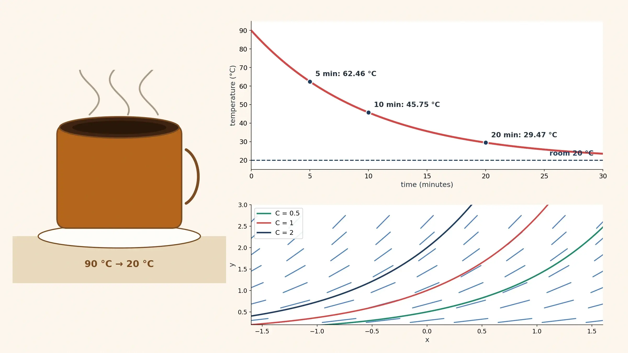
The coffee started at about 90 degrees Celsius in a room at about 20 degrees. Five minutes later it was about 62 degrees. Ten minutes in, about 46 degrees. Twenty minutes in, about 29 degrees. Notice what those numbers say. In the first five minutes the coffee lost about 28 degrees; in the next five, about 17; in the ten minutes after that, about 16. The cooling slowed down as the coffee approached room temperature, and it slowed in a regular way: the hotter the coffee, the faster it cooled. That is not a vague impression. It is a rule, and the rule can be written as an equation about a rate.
The rule has a name. Newton published it anonymously in 1701, in a paper called Scala graduum Caloris in the Philosophical Transactions of the Royal Society of London. The rate of cooling of a body is proportional to the difference between its temperature and the temperature of its surroundings. Hot coffee in a cool room cools fast. Lukewarm coffee in the same room cools slowly. The rule says nothing about the coffee being coffee. It says something about how a difference shrinks, and the same shrinking appears in circuits, in drug clearance, and in radioactive decay.
The rate depends on the temperature itself
Here is the turn that makes differential equations interesting. The rate of change of the temperature depends on the temperature itself, right now. That sounds circular, and in a sense it is: to know how fast the coffee is cooling, you need to know how hot it is, and how hot it is depends on how fast it has been cooling. The equation does not hand you the temperature. It hands you the rule that the temperature must obey at every instant, and the job of solving the equation is to find the function — the whole cooling curve — that obeys the rule everywhere.
I timed a mug once with a kitchen thermometer and a notebook, taking a reading every minute for half an hour, because I wanted to see whether the rule was real or just a textbook story. The readings fell fast, then slower, then slower still, and when I plotted them the points sat on a smooth curve that bent exactly the way the rule said it should. The surprise was not that the numbers matched. The surprise was how ordinary the experiment felt: a mug, a thermometer, a clock, and a curve that knew where it was going before I did. That is what differential equations do: they turn a sequence of measurements into a prediction.
From a cup to a language
The coffee is only the doorway. The same pattern — the rate of change depending on the current state — appears wherever something changes. A population grows faster when there are more individuals to reproduce. A predator population grows when prey are plentiful and shrinks when they are scarce. A capacitor charges fast when it is empty and slowly as it fills. An epidemic grows fast when many people are still susceptible and slows as immunity builds. A planet accelerates toward the Sun more strongly when it is closer, so its motion is a rule about how position changes, written in terms of position itself. The same language — differential equations — describes them all.
2. What Are Differential Equations?
Differential equations are equations that link a function to its derivatives. That is the whole definition, and it is worth sitting with for a moment, because everything else in this article about differential equations is a consequence of it. A differential equation does not ask for a number. It asks for a function: a rule that gives a value at every moment, or at every point, and whose rates of change fit the equation. Solving differential equations means finding that function. The answer to a differential equation is a curve, not a number, and the curve is the story of how something changes.
An equation about a rate, not a number
The symbols are less frightening than they look. Write T for the temperature of the coffee and t for time. Then dT/dt means the rate at which T changes as t passes: the slope of the temperature curve. Newton's cooling rule becomes dT/dt equals minus k times the difference between T and room temperature, where k is a positive number that says how fast heat escapes. The minus sign says the temperature falls while it stands above room temperature. The letter k carries the physics: a thin-walled cup in a draught has a larger k than a thick insulated flask.
Derivatives and integrals are the tools differential equations are built from, and they are explained from the ground up in our article on how calculus works. This article uses them and does not re-teach them. What matters here is the new step: putting derivatives inside an equation, and asking which function makes it true.
The answer is a whole family
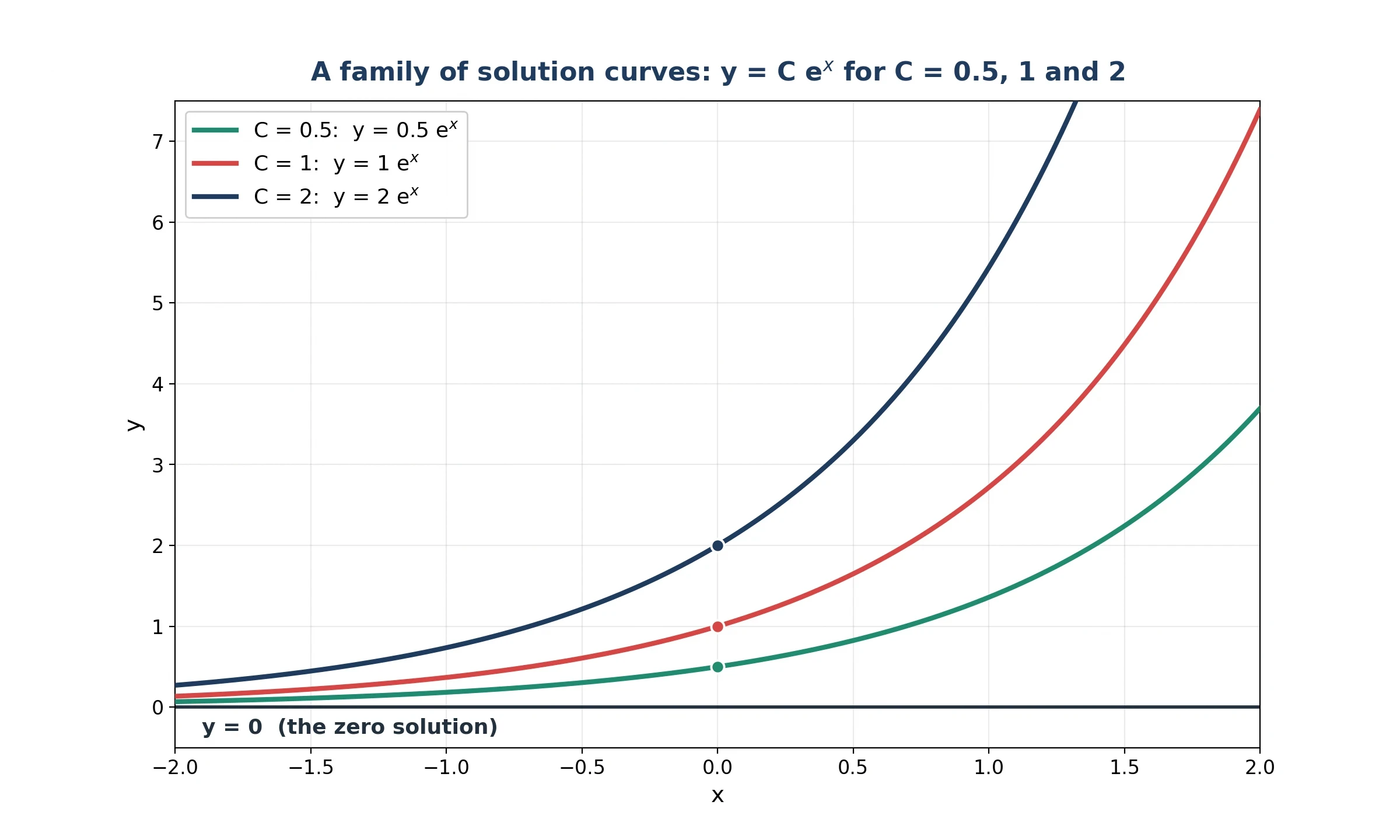
One differential equation usually has many solutions, not one. Take the simplest differential equation there is: dy/dx equals y. It says the rate of change of y equals y itself. The function y equals e to the power x satisfies it, because the derivative of e to the power x is e to the power x — and so does y equals any constant C times e to the power x. Each choice of C gives a different curve, and all of them satisfy the same equation. The general solution is a family of curves, and the constant C picks one member of the family.
The equation alone does not choose a curve. It chooses a family, a whole set of curves obeying the same rule about slopes. To pick one curve out of the family, you need one more piece of information, a starting value, and that is the subject of section 5.
Why "differential equations" is the right name
The name says what the subject is. "Differential" points to the differentials — the tiny rates of change, dy and dx, that the equation is built from. "Equations" says those rates are tied together in a condition the unknown function must satisfy. Put together, differential equations are equations about rates, and their solutions are the functions whose rates fit. The name is a description, not a decoration: every differential equation in this article is an equation about how fast something changes, and every solution is the curve that changes that way.
3. Ordinary vs Partial: ODEs and PDEs
One variable changes: ordinary differential equations
An ordinary differential equation involves an unknown function of only one variable, and ordinary derivatives of that function. The cooling equation is one: temperature T depends on time t alone, and the equation involves dT/dt, an ordinary derivative. The population equation is another: population P depends on time alone, and dP/dt equals r times P says the population grows in proportion to its size. The charge on a capacitor depends on time alone, so its equation is an ODE too. One variable changes, one story unfolds, and the solution is a curve: a single line that can be drawn on a flat page.
Ordinary differential equations are the half of differential equations this article spends most of its time on, because they are the half that can be solved most often. The definitions in this section follow the classification in the LibreTexts introduction to differential equations, which sets out ODEs, PDEs, order, linearity, and homogeneity in one place. Sections 6, 7, and 8 tour the standard methods for ODEs: separation of variables, integrating factors, and the characteristic equation. Each method fits a particular shape of equation, and part of learning differential equations is learning to recognise the shape at a glance. An ODE describes a single unfolding story — a cup cooling, a population growing, a spring swinging — and the story has a beginning, a middle, and an end that the equation predicts.
Several variables change: partial differential equations
A partial differential equation involves partial derivatives of a function of more than one variable. The temperature in a metal bar is the classic example: it depends on position x along the bar and on time t, so it is a function of two variables, and its equation involves partial derivatives — rates of change with one variable held still while the other moves. The heat equation says the rate at which the temperature changes in time is proportional to how sharply it varies in space. The wave equation says the acceleration of a point on a string depends on how sharply the string curves in space. Both are PDEs, and both need a surface, not a curve, to draw their solutions.
Partial differential equations describe fields spread over space and time: temperature fields, displacement fields, electric potentials, quantum wave functions. Their solutions are landscapes, not lines: a hot spot in the middle of a bar spreads outward, a plucked string sends waves in both directions, and a steady electric potential settles into a smooth shape with no bumps. The mathematics is harder, and exact solutions are rarer, but the ideas are the same: the equation is a rule about rates, and the solution is the shape that obeys the rule everywhere.
Why the split matters
The split matters because the two kinds of equation behave differently. In differential equations, an ODE with a starting value usually has exactly one solution, as section 5 explains. A PDE needs more: a starting shape over the whole region, plus conditions at the boundaries — the ends of the bar held at fixed temperatures, for example. Change the boundary conditions and you change the solution, even when the equation stays the same. A violin string and a guitar string obey the same wave equation, but their different lengths give different notes, because the boundary conditions differ.
The same world, two kinds of equation
The two kinds behave differently, but they describe the same world, and the same physical situation can need both. A cooling cup is an ODE while its temperature is uniform, and becomes a PDE the moment the temperature varies from point to point inside the cup. A vibrating string is a PDE in space and time, and each of its modes is an ODE in time alone. The split is a choice of viewpoint, not a wall between subjects: the equation follows the question, and the question decides how many variables the answer needs.
4. Order, Linearity, and the Language of Classification
Order: how deep the derivatives go
The order of a differential equation is the order of the highest derivative that appears in it. A first-order equation involves only first derivatives: dy/dx equals y is first order, and so is the cooling equation. A second-order equation involves a second derivative: the spring equation, m times x double-prime plus k times x equals 0, is second order because acceleration is the second derivative of position. The order counts how deep the derivatives go, and something else too: a general solution of an nth-order equation contains n free constants, so a second-order equation needs two starting values, not one.
Linear or nonlinear: can you add solutions?
A linear differential equation is one in which the unknown function and its derivatives appear only to the first power, never multiplied together, and never inside another function. The equation y double-prime minus 3y prime plus 2y equals 0 is linear, and so is dy/dx equals y. The equation dy/dx equals y squared is not linear, because y appears squared, and dy/dx equals sin y is not linear, because y sits inside a sine. The test is mechanical, and it matters, because linear equations have a property that nonlinear ones do not: superposition. If two functions both solve a linear homogeneous equation, then any combination of them — any sum, any multiple — solves it too. That is why the general solution of a linear equation is built by adding basic solutions together, and why section 8 can build the spring solution out of exponentials.
Nonlinear equations do not allow that. The Lotka-Volterra predator-prey equations are nonlinear, because they contain the product of prey and predator populations, and their solutions cannot be added together to make new solutions. The logistic equation is nonlinear too, because it contains N squared in disguise: dN/dt equals r times N times one minus N over K expands to a term in N squared. Nonlinear does not mean unsolvable. It means the superposition trick fails, the solution set is not built by adding pieces, and the behaviour can be richer — cycles, thresholds, sudden changes — than any linear equation can produce.
Homogeneous or not, constant coefficients or not
The remaining labels are smaller, but they decide the method. A linear equation is homogeneous if every term depends on the dependent variable — that is, there is no term that is a function of the independent variable alone. The equation y double-prime minus 3y prime plus 2y equals 0 is homogeneous. Add a term like e to the power x on the right-hand side, and it becomes non-homogeneous: the equation is now driven by an outside force, and the solution gains a particular part that follows it. Constant coefficients means the coefficients are constant numbers, not functions of the independent variable. The equation y double-prime minus 3y prime plus 2y equals 0 has constant coefficients, and that is why the characteristic equation method of section 8 works on it. Let the coefficients vary with x, and the method fails.
| Equation | ODE or PDE | Order | Linear or nonlinear | What it models |
|---|---|---|---|---|
| dy/dx equals y | ODE | First | Linear | Exponential growth and decay |
| dP/dt equals 0.03 times P | ODE | First | Linear | A population growing at 3 percent per year |
| y double-prime minus 3y prime plus 2y equals 0 | ODE | Second | Linear | The characteristic-equation example of section 8 |
| Lotka-Volterra predator-prey equations | ODE system | First | Nonlinear | Predator and prey populations cycling |
| Heat equation | PDE | Second | Linear | Temperature spreading along a rod |
| Wave equation | PDE | Second | Linear | A vibrating string |
Table 1: Classification at a glance. Six example differential equations, each labelled ODE or PDE, order, linear or nonlinear, and what it models.
Why mathematicians classify first
Classification chooses the method in differential equations. A first-order linear equation gets an integrating factor, as section 7 shows. A separable equation gets separation of variables, as section 6 shows. A second-order linear equation with constant coefficients gets the characteristic equation, as section 8 shows. A nonlinear equation gets a phase plane, or a numerical method, as sections 13 and 14 show.
5. The First Question: Does a Solution Exist?
A slope field: the whole solution family at a glance
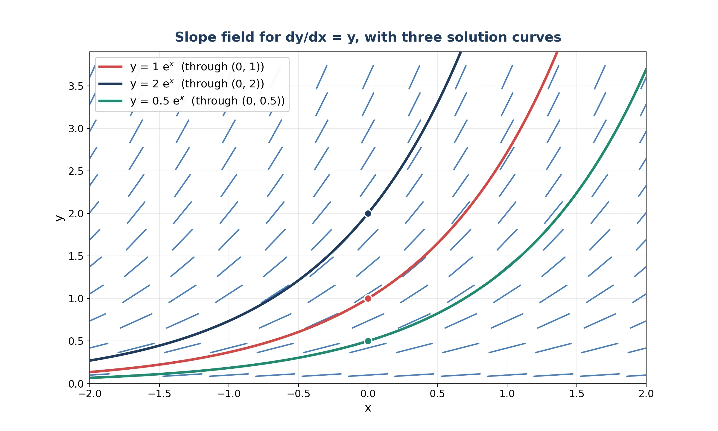
A slope field is the most direct picture in differential equations. Take the equation dy/dx equals y. At every point of the plane, the equation says what the slope of a solution must be there: where y is 1, the slope is 1; where y is 2, the slope is 2; where y is negative, the slope is negative. Draw a short line segment at each point with the slope the equation demands, and the segments line up into visible flows, like iron filings around a magnet. A solution curve follows the segments, threading through them, always going in the direction they point. Three solution curves are drawn through it, starting at the points where x is 0 and y is 1, 2, and 0.5.
I sketched a slope field by hand once, on squared paper, for an equation I did not yet know how to solve, marking a little segment at each grid point and then trying to draw a curve that followed them. The first attempt wandered off the segments and looked wrong at once; the second followed them, and the curve that emerged bent in a way I had not predicted. It was the first time I understood that a differential equation is a set of instructions for drawing, and that the drawing is the solution.
Initial conditions pick one curve
The same equation with a different starting point gives a different story. That is the initial value problem: the differential equation plus the value of the unknown at one starting point, and the question is which member of the family passes through that point. For dy/dx equals y, the starting value y of 0 equals 1 picks y equals e to the power x, y of 0 equals 2 picks y equals 2 times e to the power x, and y of 0 equals 0 picks the flat zero curve. The equation is the rule; the initial condition is the choice.
Picard and Lindelöf, 1890 and 1894
In differential equations, under reasonable conditions, exactly one solution passes through each starting point. That is the content of the Picard-Lindelöf theorem, proved in its modern form by Émile Picard in 1890, in a memoir on the theory of differential equations published in the Journal de l'École Polytechnique, and by Ernst Lindelöf in 1894, in a note on successive approximations in the Comptes Rendus. The theorem concerns an initial value problem dy/dt equals F of t and y, with y of t0 equal to y0. If F is continuous and not too steep in y — the technical condition is that F is locally Lipschitz in y, and continuous differentiability is enough — then a solution exists on some interval around t0, and it is unique. One starting point, one curve, at least for a while.
When uniqueness fails
The honest caveat is that a merely continuous right-hand side guarantees existence, not uniqueness. The classic example is dy/dx equals the square root of the absolute value of y, with y of 0 equal to 0. The zero function solves it, and so does a function that stays at zero for a while and then lifts off along a parabola. The right-hand side is continuous, but it is too steep near zero in the sense the theorem cares about, and uniqueness fails. The equation has many solutions through the same starting point, and no amount of staring at the starting value will choose among them.
One starting point gives one future, when the theorem applies, and chance enters only when the model adds it. Randomness, probability, and the measurement of uncertainty belong in our article on what probability is, and the differential equations in this article are deterministic: the same start, the same rule, the same curve, every time.
6. Separation of Variables: The First Tool That Works
When the two sides can be pulled apart
The method applies to an equation of the form dy/dx equals a function of x times a function of y. Write it as dy/dx equals f of x times g of y. Divide both sides by g of y, multiply both sides by dx, and the equation becomes dy divided by g of y equals f of x times dx: the left side involves only y, the right side only x. Integrate both sides, and the two integrals are equal up to a constant. Solve for y, and the general solution appears, constant and all.
The step that worries beginners is the division by g of y, which fails where g of y is zero. Separation of variables turns differential equations of this shape into two ordinary integrals, and that is its power. It is also its limit: if the equation cannot be written as a product of a function of x and a function of y, the sides will not separate, and no amount of rearrangement will make them. The method is a first tool, not a universal one, and recognising when it applies is half the skill.
Worked example: exponential growth
Take a population P growing at 3 percent per year, starting from 1000 individuals. The equation is dP/dt equals 0.03 times P. Separate: dP divided by P equals 0.03 dt. Integrate both sides: the natural logarithm of P equals 0.03 t plus a constant. Exponentiate, and the starting value P of 0 equals 1000 fixes the constant at 1000. The solution is P of t equals 1000 times e to the power 0.03 t. After 10 years, P is 1000 times e to the power 0.3, which is 1349.86: the population has grown by about a third in a decade.
The doubling time follows from the same solution: set P equal to 2000 and solve 2 equals e to the power 0.03 t, giving t equal to the natural logarithm of 2 divided by 0.03, or 23.10 years. That number does not depend on the starting population: a thousand doubles in 23.10 years, and so does a million, because the growth is proportional. The step that turns e to the power k t into a doubling time is a logarithm, and the rules of logarithms are set out in our article on what a logarithm is. This article uses logarithms; it does not re-teach them.
Worked example: the logistic equation
The logistic equation is solved the same way, and it is a better advertisement for the method, because the integration is harder and the answer is more interesting. Separate: dN divided by N times one minus N over K equals r dt. The left side splits by partial fractions, each term integrating to a logarithm, and the result, after algebra, is the logistic function: N of t equals K divided by one plus A times e to the power minus r t, where A equals K minus N0 all divided by N0.
The solution checks out exactly: differentiating the logistic function and substituting it back gives a residual of exactly zero. A claimed solution is not a solution until it survives substitution, and the logistic solution survives it cleanly.
Where separation fails
Most equations do not separate, and it is worth saying so plainly. The equation dy/dx equals x plus y does not separate, because the right side is a sum, not a product of a function of x and a function of y. The equation dy/dx equals sin of x times y plus y squared does not separate either. No rearrangement will pull the variables apart, because the equation mixes them in a way that separation cannot undo. The first step in solving is to look at the shape, and to reach for separation only when the shape fits.
7. Integrating Factors and Linear First-Order Equations
The linear first-order shape
The shape is dy/dx plus P of x times y equals Q of x, where P and Q are known functions of x. The term P of x times y is the self-referential part — the rate of change depends on y itself — and Q of x is the driving part, an outside influence that does not depend on y. When Q is zero, the equation is homogeneous and separates. When Q is not zero, the driving term tangles the sides, and the integrating factor is the tool that untangles it.
The history of the integrating factor is a small lesson in how differential equations actually developed. Johann Bernoulli had the idea in lecture notes prepared in the early 1690s, published only in 1742, long after the idea had circulated. Euler developed the full theory in a paper published in 1741, working on the exactness of first-order equations and integrating factors in the 1730s. Bernoulli had the idea first, in notes that stayed unpublished; Euler built the theory that everyone learned.
The multiplying trick
Multiply the whole equation by a well-chosen function mu of x, called the integrating factor, and the left side collapses into a single derivative. Choose mu equal to e to the power of the integral of P of x dx: then the derivative of mu times y, by the product rule, is exactly mu times the left side of the equation. The equation becomes d/dx of mu times y equals mu times Q of x. Integrate both sides, divide by mu, and the solution appears: y equals one over mu times the integral of mu times Q of x dx, plus a constant over mu.
I remember the afternoon the trick first clicked for me, working through a messy equation whose left side looked hopeless, with a y term and a derivative tangled together in a way that separation could not touch. I multiplied through by the exponential factor, watched the two terms fold into a single derivative of a product, and felt a small, disproportionate satisfaction. That is the whole pleasure of the integrating factor in differential equations: it does not fight the equation, it reframes it, and the reframe makes the answer obvious.
Worked example
Take the equation y prime plus 2y equals e to the power minus x. Here P of x is 2, a constant, and Q of x is e to the power minus x. The integrating factor is mu equals e to the power of the integral of 2 dx, which is e to the power 2x. Multiply through: e to the power 2x times y prime plus 2 times e to the power 2x times y equals e to the power x. The left side is the derivative of e to the power 2x times y, so integrate: e to the power 2x times y equals e to the power x plus C. Divide by e to the power 2x: y equals e to the power minus x plus C times e to the power minus 2x. The solution checks exactly: substituting it into y prime plus 2y minus e to the power minus x gives zero.
Put a starting value on it. With y of 0 equal to 3, the solution gives 3 equals 1 plus C, so C equals 2, and y equals e to the power minus x plus 2 times e to the power minus 2x. At x equal to 1, y is e to the power minus 1 plus 2 times e to the power minus 2, which is 0.3679 plus 0.2707, giving 0.6386. Two exponentials compete in that answer: one decaying at rate 1, driven by the right-hand side, and one decaying at rate 2, carrying the memory of the starting value. That is the shape of a linear first-order solution in general: a driven part that follows the outside force, plus a transient part that carries the starting value and fades away.
The Bernoulli equation, 1695
The Bernoulli equation is a famous near-miss for the linear method: a change of variable can turn a nonlinear equation into a linear one. Jacob Bernoulli proposed it in December 1695, in the Acta Eruditorum, and set it as a challenge: y prime plus P of x times y equals Q of x times y to the power n, where n is a number other than 0 or 1. The equation is nonlinear, because of the y to the power n term, and the linear method does not apply directly. Leibniz showed in 1696 that it reduces to a linear equation with the change of variable z equals y to the power 1 minus n. Johann Bernoulli gave another method, and Jacob Bernoulli solved it by separation of variables. Three solutions, three routes, one equation — and the credit belongs to all of them.
8. Second-Order Equations and the Characteristic Equation
Why second order needs two starting values
Second-order differential equations need two starting values, because their general solutions contain two free constants. For a spring, the two values are position and velocity: where the mass is when you start the clock, and how fast it is moving. Give both, and the motion is fixed for all time; give only the position, and the mass could be sitting still or flying through that position at speed. The mathematics matches the physics: a second derivative is a rate of change of a rate of change, and to pin down a curve with a prescribed curvature at every point, you must pin down where it starts and how steeply it leaves.
The characteristic equation
Take y double-prime plus a times y prime plus b times y equals 0, with a and b constant, and assume a solution of the form y equals e to the power r x, for some number r to be found. Then y prime is r times e to the power r x, and y double-prime is r squared times e to the power r x. Substitute: r squared plus a times r plus b, all times e to the power r x, equals 0. Since e to the power r x is never zero, the bracket must be zero: r squared plus a r plus b equals 0 — the characteristic equation, an ordinary quadratic, whose roots decide the shape of the solution. Euler knew the exponential ansatz as early as 1739, in correspondence with Johann Bernoulli, and published the full treatment of higher-order linear equations with constant coefficients in 1743, in a paper on the integration of differential equations of higher degree.
Worked example
Take y double-prime minus 3y prime plus 2y equals 0. The characteristic equation is r squared minus 3r plus 2 equals 0, which factors as r minus 1 times r minus 2 equals 0, so the roots are 1 and 2. The general solution is y equals C1 times e to the power x plus C2 times e to the power 2x. The solution checks exactly: substituting it into the equation gives zero. Now impose starting values: y of 0 equal to 3, and y prime of 0 equal to 5. At x equal to 0, y is C1 plus C2, so C1 plus C2 equals 3. The derivative is C1 times e to the power x plus 2 C2 times e to the power 2x, so at x equal to 0 it is C1 plus 2 C2, which equals 5. Subtracting gives C2 equals 2, and C1 equals 1. The particular solution is y equals e to the power x plus 2 times e to the power 2x, and at x equal to 1 it is e plus 2 times e squared, which is 2.7183 plus 14.7781, giving 17.4964.
Complex roots and oscillation
In differential equations, complex roots give oscillation, and the spring is the reason this matters. Take y double-prime plus 2y prime plus 5y equals 0. The characteristic equation is r squared plus 2r plus 5 equals 0, whose roots are minus 1 plus or minus 2i. The solution is y equals e to the power minus x times cos 2x, up to constants, and it checks exactly. The shape is a cosine wave wrapped in a decaying exponential: the mass oscillates with frequency 2, and the amplitude shrinks by a factor of e to the power minus x. That is damped oscillation, the motion of a real spring losing energy to friction, and it is the shape that makes the characteristic equation worth learning.
The complex numbers in that solution are not a decoration. They are the machinery that turns a quadratic with no real roots into a real oscillation, and the rules for handling them — the complex plane, Euler's formula, the meaning of i — are set out in our article on imaginary numbers. This article uses complex roots; it does not re-teach them. What matters here is the correspondence: a pair of complex roots means oscillation, the real part means growth or decay, and the imaginary part means frequency.
Repeated roots and the extra x
When the characteristic quadratic has one root twice, the second solution gains a factor of x. Take y double-prime minus 2y prime plus y equals 0: the characteristic equation is r squared minus 2r plus 1 equals 0, which is r minus 1 squared, so the root is 1, twice. One solution is e to the power x. The second solution is x times e to the power x, and the general solution is y equals C1 times e to the power x plus C2 times x times e to the power x. The extra x is not a guess: it comes from the method of reduction of order, which builds a second solution from the first when the two roots coincide.
9. Newton's Second Law as a Differential Equation
F equals m a, rewritten as a differential equation
Write x for position and t for time. Velocity is dx/dt, the first derivative of position. Acceleration is the second derivative, d squared x over dt squared, as defined in our article on how calculus works. Newton's second law says the acceleration of a mass m under a force F is F divided by m, so the equation is m times d squared x over dt squared equals F. The force F may depend on position, on velocity, or on time, and each dependence gives a different equation. A constant force gives constant acceleration, a force proportional to position gives oscillation, and a force proportional to velocity gives damping. Each dependence gives a different member of the family of differential equations that Newton's law generates.
The spring: simple harmonic motion
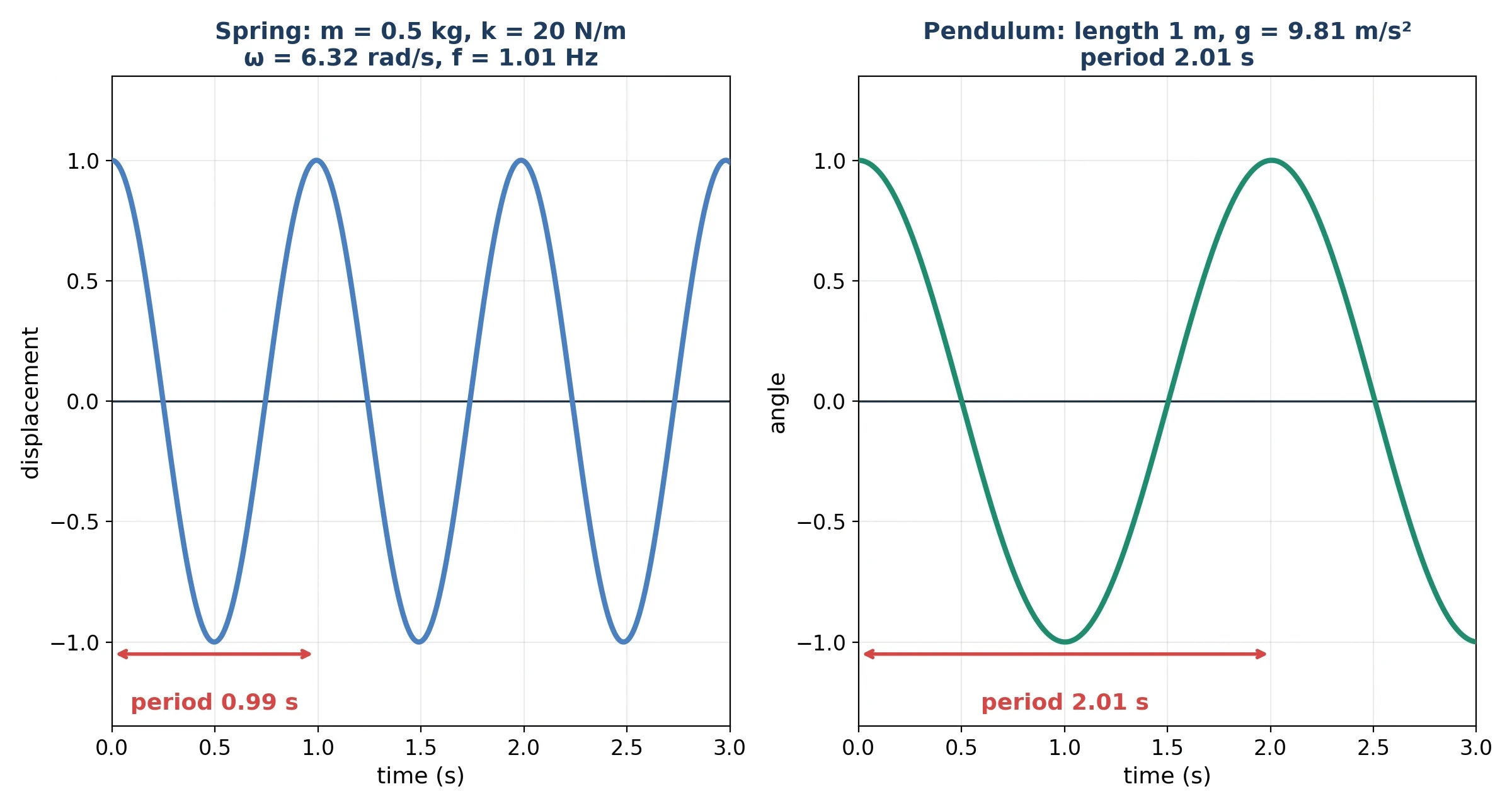
A mass on a spring is the cleanest second-order equation in physics. Hooke's law says the spring pulls back with a force proportional to how far it has been stretched: F equals minus k times x, where k is the spring constant and the minus sign says the force points back toward rest. Newton's second law gives m times x double-prime equals minus k times x, or x double-prime plus k over m times x equals 0. The solution is an oscillation: x equals A cos of omega t, where omega equals the square root of k over m, and A is the amplitude.
Put numbers on it: a mass of 0.5 kilograms on a spring with spring constant 20 newtons per metre gives omega equal to the square root of 20 divided by 0.5, or 6.3246 radians per second. The period is 2 pi divided by omega, or 0.9935 seconds — just under one second per swing — and the frequency is 1.007 hertz. The solution checks exactly: y equals A cos of omega t satisfies y double-prime plus omega squared times y equals 0.
The pendulum
A pendulum is a spring in disguise, with gravity doing the work of the spring: a bob of mass m hangs from a string of length L, and gravity pulls it back toward the bottom with a force proportional to the sine of the angle. For small angles, the sine of the angle is close to the angle itself, and the equation becomes the same as the spring: angle double-prime plus g over L times angle equals 0, where g is 9.81 metres per second squared. The period is 2 pi times the square root of L over g. For a pendulum of length 1 metre, the period is 2 pi times the square root of 1 divided by 9.81, or 2.006 seconds: just over two seconds per swing.
The small-angle approximation holds only while the angle stays small. Swing a pendulum through a wide arc, and the sine and the angle part company, and the period grows: a pendulum swinging through 60 degrees takes longer than the small-angle formula says, and the exact period needs an integral with no elementary form. The approximation is a working tool, not a law of nature, and the place where it breaks is a reminder that every model has a range.
I once counted a pendulum against a stopwatch, a length of string with a fishing weight on the end, swinging beside a kitchen clock, timing ten swings and dividing by ten to steady the count. The measured period came out within a few hundredths of a second of the formula. Then I pulled the bob wider, and the period stretched, just as the theory said it would. That is the feeling differential equations give at their best: a formula that earns its keep, and a failure that teaches as much as the success.
Free fall, with numbers
Free fall is the simplest case of all: a constant force, gravity, and no other forces. The equation is x double-prime equals g, with g equal to 9.81 metres per second squared downward. Integrate once: velocity equals g times t, starting from rest. Integrate again: distance equals one half times g times t squared. After 3 seconds of falling with no air resistance, the velocity is 9.81 times 3, or 29.43 metres per second, and the distance fallen is one half times 9.81 times 9, or 44.15 metres.
Why Newton needed a new mathematics
Newton needed differential equations because his laws are rules about change, and change is what derivatives measure. His three laws describe how velocity changes under force, but none of them predicts anything until the second law is written as a differential equation and solved, and the solving needed the calculus that Newton had developed in manuscripts from 1665 to 1666 and Leibniz had published in 1684. The Principia presented the laws in geometrical form, but the equations underneath were differential, and the two centuries of mechanics that followed worked out their solutions.
10. Population Growth: Exponential, Then Logistic
Malthus, 1798
Thomas Robert Malthus published An Essay on the Principle of Population anonymously in 1798, and its argument was stark. Population, unchecked, grows in geometric progression: it doubles, doubles again, and doubles again. Food, he argued, grows only in arithmetic progression: it adds a fixed amount each year. A geometric progression outruns an arithmetic one, and the gap between them is famine, disease, and war — the checks that bring a population back in line. He claimed population doubles about every 25 years, and the growth rate implied by a 25-year doubling time is the natural logarithm of 2 divided by 25, or 0.02773 per year: e to the power 0.02773 times 25 is 2.0000, exactly the doubling the claim requires.
Malthus's point was not that populations double every 25 years forever. His point was that they cannot, and that something must stop them. A population growing at 2.773 percent per year would cover the Earth in a few centuries, and it does not, because the world pushes back. The pushback is the subject of the next two sections. Malthus's argument later shaped Darwin's thinking about the struggle for existence, as our article on natural selection explains, and the populations he described are the populations whose branching history is drawn in our article on the tree of life.
Exponential growth, worked
The exponential model is one of the simplest differential equations: dP/dt equals r times P, solved in section 6, with P0 equal to 1000 and r equal to 0.03 per year giving P at 10 years of 1349.86 and a doubling time of 23.10 years. A single number, r, predicts the whole future — and that is also its limit: nothing real grows exponentially forever, because nothing real has unlimited food, space, or time.
Verhulst, 1838, and the carrying capacity
Pierre-François Verhulst, a Belgian mathematician, published the correction in 1838, in the Correspondance Mathématique et Physique, volume 10, pages 113 to 121. The logistic equation is one of the most famous differential equations in biology: dN/dt equals r times N times one minus N over K, where r is the intrinsic growth rate and K is the carrying capacity: the largest population the environment can support. The new term, one minus N over K, is the brake: when N is small compared with K, the brake is close to 1 and the population grows almost exponentially; when N approaches K, the brake approaches zero and growth stops; when N exceeds K, the brake goes negative and the population shrinks back toward K. The equation contains its own limit, and that is its genius.
The carrying capacity is not a law of nature. It is a summary of food, habitat, climate, predators, and disease, all rolled into one number, and in a real ecosystem that number moves. The logistic equation assumes a constant K, and that assumption is rarely true in practice: food, habitat, climate, predators, and disease all move K, sometimes fast. The model is a starting point, not a forecast: it names the brake and shows its shape.
The S-curve, worked
Take K equal to 1000, a starting population of 100, and a growth rate r equal to 0.5 per unit time. The constant A equals K minus N0 all divided by N0, which is 900 divided by 100, or 9. The solution is N of t equals 1000 divided by one plus 9 times e to the power minus 0.5 t: at time 0 it is 100, at time 2 it is 231.97, at time 5 it is 575.12, and at time 10 it is 942.83.
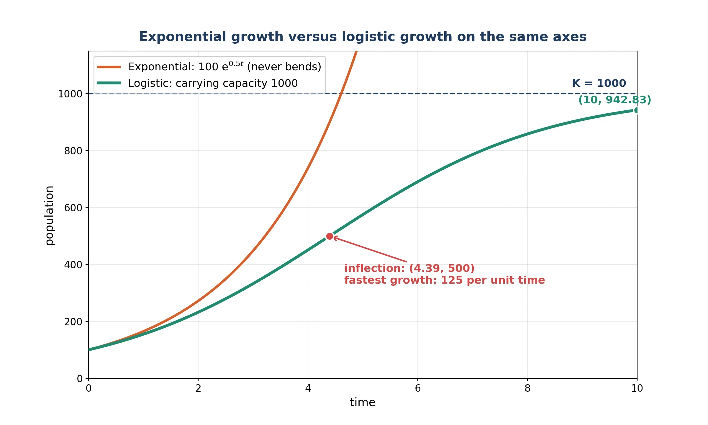
The inflection point is where the curve changes from bending upward to bending downward — and where growth is fastest. It sits at N equal to K over 2, which is 500, and it is reached at time equal to the natural logarithm of A divided by r, which is the natural logarithm of 9 divided by 0.5, or 4.3944. The fastest growth rate is r times K over 4, which is 0.5 times 1000 over 4, or 125 per unit time, and the derivative at N equal to 500 confirms it: dN/dt at 500 is exactly 125.0. Before the inflection, growth accelerates as the population grows; after it, growth decelerates as the brake tightens.
Pearl and Reed rediscover the logistic curve in 1920; Lotka gives a rational explanation in 1925
Verhulst's paper was largely ignored for more than eighty years. Then Raymond Pearl and Lowell Reed rediscovered the curve empirically in 1920, fitting it to United States population data. Alfred J. Lotka gave a rational explanation in 1925, in Elements of Physical Biology, showing how the curve follows from the dynamics of growth and limitation. The equation is also called the Verhulst-Pearl equation, and the name carries the history in it.
11. Newton's Law of Cooling and the RC Circuit
Newton's cooling law, 1701
Newton published his cooling law anonymously in March to April 1701, as Scala graduum Caloris in the Philosophical Transactions of the Royal Society of London, volume 22, pages 824 to 829. The law says the rate of heat loss of a body is directly proportional to the difference in temperatures between the body and its environment. As a differential equation, dT/dt equals minus k times the difference between T and the environment temperature, where k is a positive constant that depends on the body and its surroundings. The solution is exponential decay of the temperature difference: the difference shrinks by the same fraction in every equal interval of time, and the temperature approaches the environment temperature without ever quite reaching it.
The cooling curve, worked
Take coffee at 90 degrees Celsius in a room at 20 degrees, with k equal to 0.1 per minute. The solution is T of t equals 20 plus 70 times e to the power minus 0.1 t: at 5 minutes it is 62.46 degrees, at 10 minutes 45.75 degrees, and at 20 minutes 29.47 degrees. The numbers are the curve from section 1, now derived from the equation, and they match the story the coffee told: fast at first, slower later, always slowing as the difference shrinks.
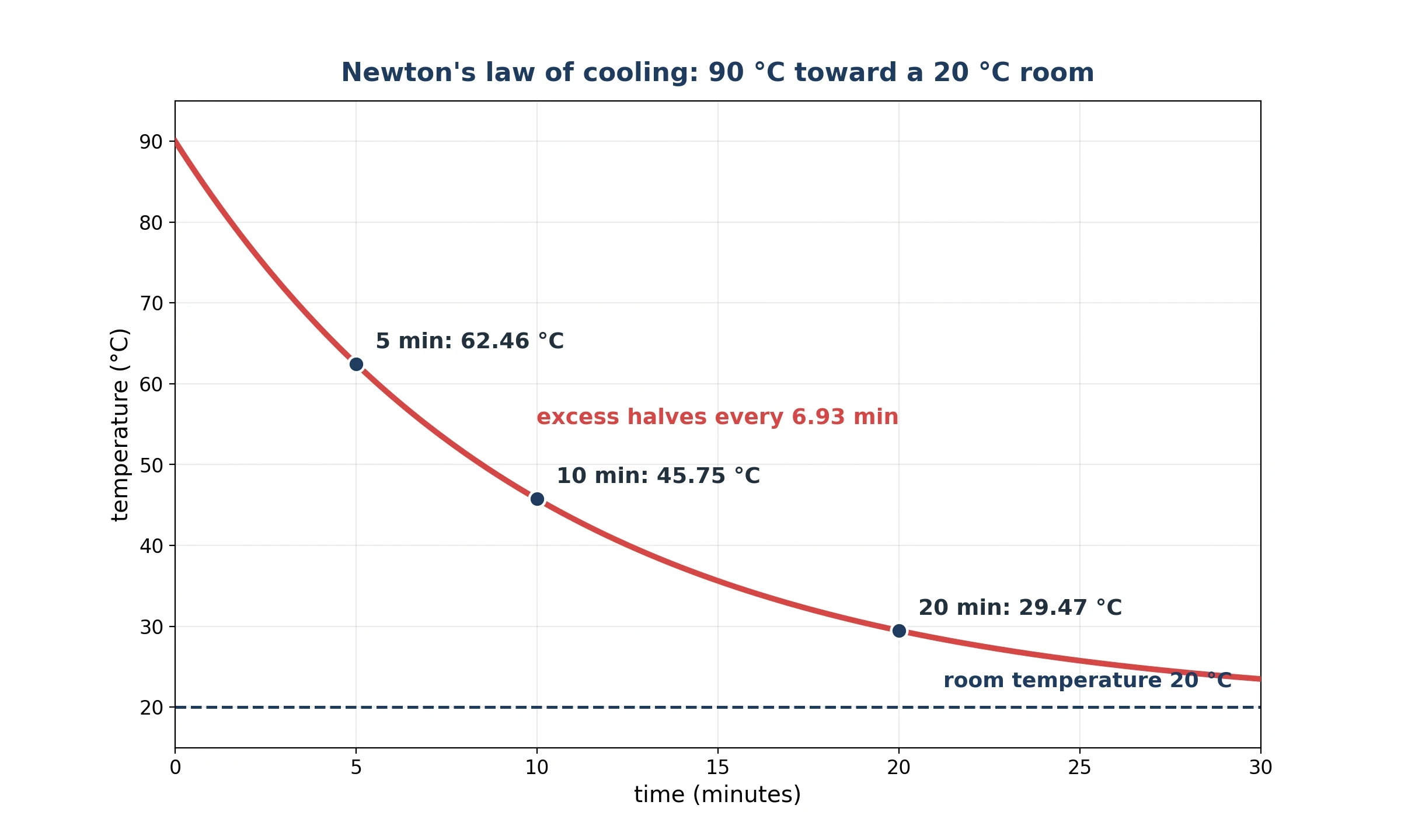
The excess over room temperature halves every 6.93 minutes, because the half-life of the excess is the natural logarithm of 2 divided by k, which is 0.6931 divided by 0.1, or 6.931 minutes. Every 6.93 minutes, the gap between the coffee and the room halves: 70 degrees, then 35, then 17.5, then 8.75, each halving taking the same time. The coffee reaches 30 degrees after 19.46 minutes, and 25 degrees after 26.39 minutes. It never reaches 20 degrees exactly, in the mathematics, though in practice it gets close enough that no thermometer can tell the difference. The law is most accurate when the temperature difference is small; for larger differences Dulong and Petit corrected it in 1817.
The same equation in a circuit
An RC circuit — a resistor and a capacitor in series — obeys one of the same differential equations as the cooling cup, and charges with the same exponential shape. The equation for the voltage V on the capacitor is dV/dt equals one over R times C times the difference between the supply voltage and V, where R is the resistance and C is the capacitance. Compare it with the cooling equation: voltage plays the role of temperature, supply voltage the role of room temperature, and one over R times C the role of k. The time constant tau equals R times C, and it plays the role of one over k: the time scale of the circuit's approach to its limit. After one time constant, 63.2 percent of the change is done. After five time constants, 99.3 percent is done.
The RC circuit, worked
Take R equal to 1000 ohms and C equal to 100 microfarads. The time constant tau equals R times C, which is 1000 times 100 times 10 to the power minus 6 seconds, or 0.100 seconds. Charging from a 12-volt supply, the voltage starts at 0 and reaches 7.585 volts after one time constant (63.2 percent of 12), 10.376 volts after two (86.5 percent), and 11.919 volts after five (99.3 percent). The fraction charged after one tau is 1 minus 1 over e, which is 0.6321, and after five tau it is 0.99326. Discharging, the voltage falls from 12 volts to 4.415 volts after one time constant, and to 1.624 volts after two.
One shape, many stories
Cooling, charging, drug clearance, radioactive decay: the same first-order differential equations govern them all, with different nouns. A drug injected into the bloodstream clears at a rate proportional to its concentration, so its concentration falls exponentially, with a half-life that doctors use to set the dose interval. A radioactive sample decays at a rate proportional to the number of atoms remaining, so its activity falls exponentially, with a half-life that archaeologists use to date the past. A capacitor charges, a cup cools, a population of bacteria dies off under an antibiotic: the equation is one, and the stories are many.
12. Heat, Waves, and the Great PDEs
D'Alembert and the vibrating string, 1747
Jean le Rond d'Alembert published the solution of the vibrating string in 1747, and it was the first solution of a partial differential equation in history. The problem was a string stretched between two fixed ends, plucked, and left to vibrate — one of the first partial differential equations ever solved. The equation says the second partial derivative of the displacement with respect to time equals a constant times the second partial derivative with respect to position: the acceleration of each point of the string depends on how sharply the string curves there. D'Alembert's solution was u of x and t equals F of x minus c t plus G of x plus c t: two waves travelling in opposite directions, each keeping its shape as it goes. Pluck a string, and two waves run away from the pluck in opposite directions, reflect from the fixed ends, and come back: the note you hear is those waves, trapped between the ends.
Fourier and the heat equation, 1822
Joseph Fourier presented his memoir on the propagation of heat to the Institut in Paris on 21 December 1807, won a prize in 1811 with a revised memoir criticised for lack of rigour, and published the book, Théorie analytique de la chaleur, in 1822. The heat equation is one of the great partial differential equations: the partial derivative of temperature with respect to time equals a constant, the diffusivity, times the second partial derivative with respect to position: temperature changes in time in proportion to how sharply it varies in space, so hot spots spread and sharp differences smooth out. Separation of variables splits the PDE into ODEs — one for space, one for time — and the solutions are modes, standing patterns that decay exponentially, each at its own rate. Fourier series follow: a wide range of initial temperature shapes can be built by adding modes together, each decaying at its own speed, so the shape smooths as it fades.
Fourier's book also contains a sentence that has been quoted ever since, because it states the creed of applied mathematics in one line.
"Profound study of nature is the most fertile source of mathematical discoveries." — Joseph Fourier, The Analytical Theory of Heat (1822), ch. 1, p. 7, trans. Alexander Freeman (1878).
Laplace and the equation of stillness, 1782
Pierre-Simon Laplace observed that the Newtonian potential satisfies Laplace's equation, in a paper on spheroids in 1782, and gave the result in Cartesian and cylindrical coordinates in a paper on Saturn's rings in 1787 — two different papers, and the result belongs to both, not to one year. Laplace's equation says the Laplacian of the potential equals zero: the sum of the second partial derivatives is zero. It governs potentials where there is no charge or mass density: the gravitational potential in empty space, the electric potential where there is no charge, the steady temperature where there are no heat sources. Where the heat equation describes change and the wave equation describes travel, Laplace's equation describes stillness: a balance with no bumps, because any bump would be smoothed away by the surrounding values.
The heat modes, worked
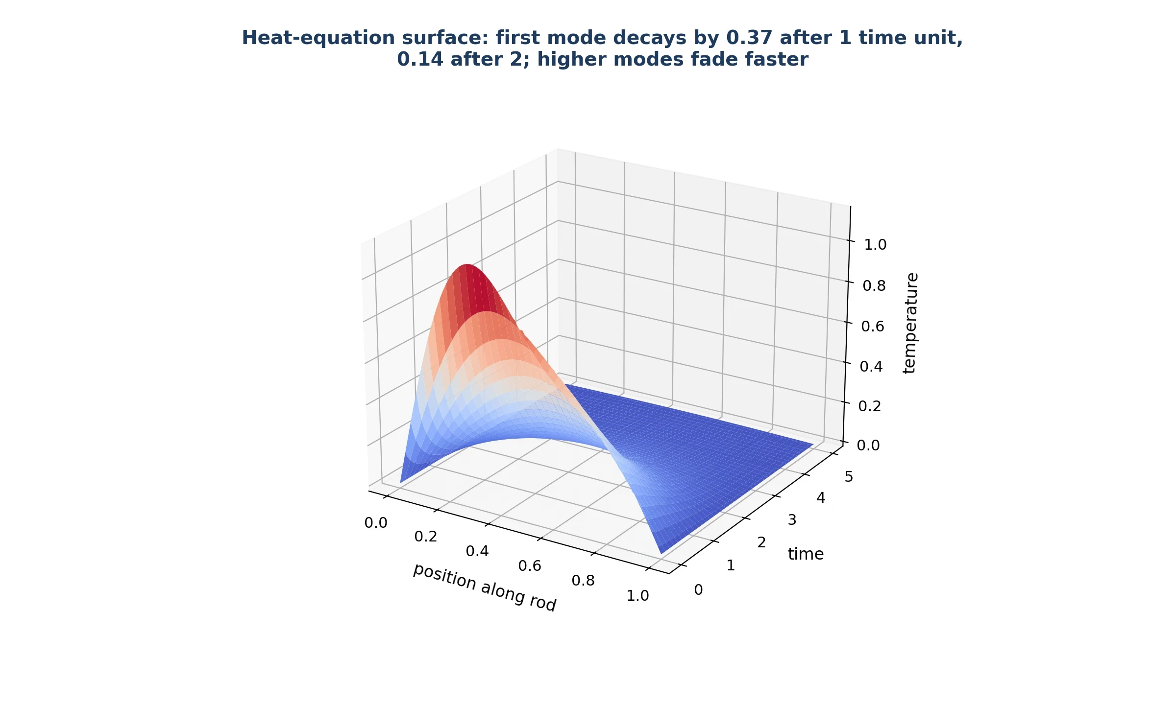
Take a rod of length 1, with diffusivity 0.1, and its first mode: a single sine wave of temperature along the rod, hot in the middle and cool at the ends. The first mode decays with rate lambda 1 equal to pi squared times 0.1 divided by 1, or 0.9870 per unit time, and its half-life is the natural logarithm of 2 divided by 0.9870, or 0.702 time units. The amplitude factor is 1.0000 at time 0, 0.3727 at time 1, 0.1389 at time 2, and 0.0072 at time 5. The second mode decays four times as fast, with lambda equal to 3.948, and the third mode nine times as fast: sharper wiggles fade faster, which is why heat smooths shapes — the fine detail disappears first, and the broad shape lingers longest.
Schrödinger, 1926, in one paragraph
Erwin Schrödinger postulated his equation in 1925 and published it in 1926, and it is a linear PDE and the quantum counterpart of Newton's second law. Where Newton's law says how a particle's position changes, Schrödinger's equation says how a quantum wave function changes, and the hydrogen spectral energies follow from it. He won the Nobel Prize in Physics in 1933 for this work; Max Born gave the probability interpretation in 1926. It belongs here as one paragraph, not as a quantum mechanics lesson: it is the proof that the language of differential equations extends from planets to electrons, and that the same move — write the rate, solve the equation — works at every scale.
| Equation | Type | Equation shape | First solver and year | Signature behaviour |
|---|---|---|---|---|
| Heat equation | Parabolic | First time derivative equals diffusivity times second space derivative | Fourier, 1822 | Smooths and fades; hot spots spread and disappear |
| Wave equation | Hyperbolic | Second time derivative equals wave speed squared times second space derivative | D'Alembert, 1747 | Travels and keeps its shape; waves run and reflect |
| Laplace equation | Elliptic | Sum of second space derivatives equals zero | Laplace, 1782 | Still and balanced; no bumps, no sources, pure smoothness |
Table 2: The three great partial differential equations compared. Heat smooths and fades, the wave travels and keeps its shape, and Laplace's equation describes stillness.
13. Living Systems: Predator and Prey, Then Epidemics
Lotka and Volterra, 1925 and 1926
Alfred J. Lotka published Elements of Physical Biology in 1925, with the predator-prey analysis inside it, and Vito Volterra published his paper independently in 1926, in Nature, volume 118, pages 558 to 560, prompted by his son-in-law-to-be Umberto D'Ancona's fish-catch data from the Adriatic. Lotka came from chemistry and the theory of oscillations. Volterra came from the fish markets of the Adriatic, where the fraction of predatory fish rose during the war years, when fishing stopped, and fell again when fishing resumed. The Lotka-Volterra equations are first-order nonlinear differential equations: dx/dt equals alpha times x minus beta times x times y, and dy/dt equals delta times x times y minus gamma times y, where x is the prey, y is the predator, alpha is the prey growth rate, beta is the predation rate, delta is the predator's gain from eating, and gamma is the predator death rate.
The history is set out in the PMC article on Lotka and the origins of theoretical population ecology, and Volterra's own paper is in Nature, volume 118, pages 558 to 560 (1926). Georgy Gause tested Volterra's conclusions experimentally in the 1930s, with protozoa in test tubes, and the cycles appeared, imperfectly, as the equations said they should.
The equilibrium, worked
With the worked parameters alpha equal to 1.0, beta equal to 0.1, delta equal to 0.05, and gamma equal to 0.5, the equilibrium sits at prey x star equal to gamma divided by delta, or 10.0, and predator y star equal to alpha divided by beta, or 10.0. At that point both rates of change are exactly zero: births balance deaths on both sides, and the populations sit still. Nudge the system away from equilibrium, and it does not return: it circles around it, in closed loops in the phase plane, prey rising, predators rising after them, prey falling, predators falling after them, and the cycle repeating.
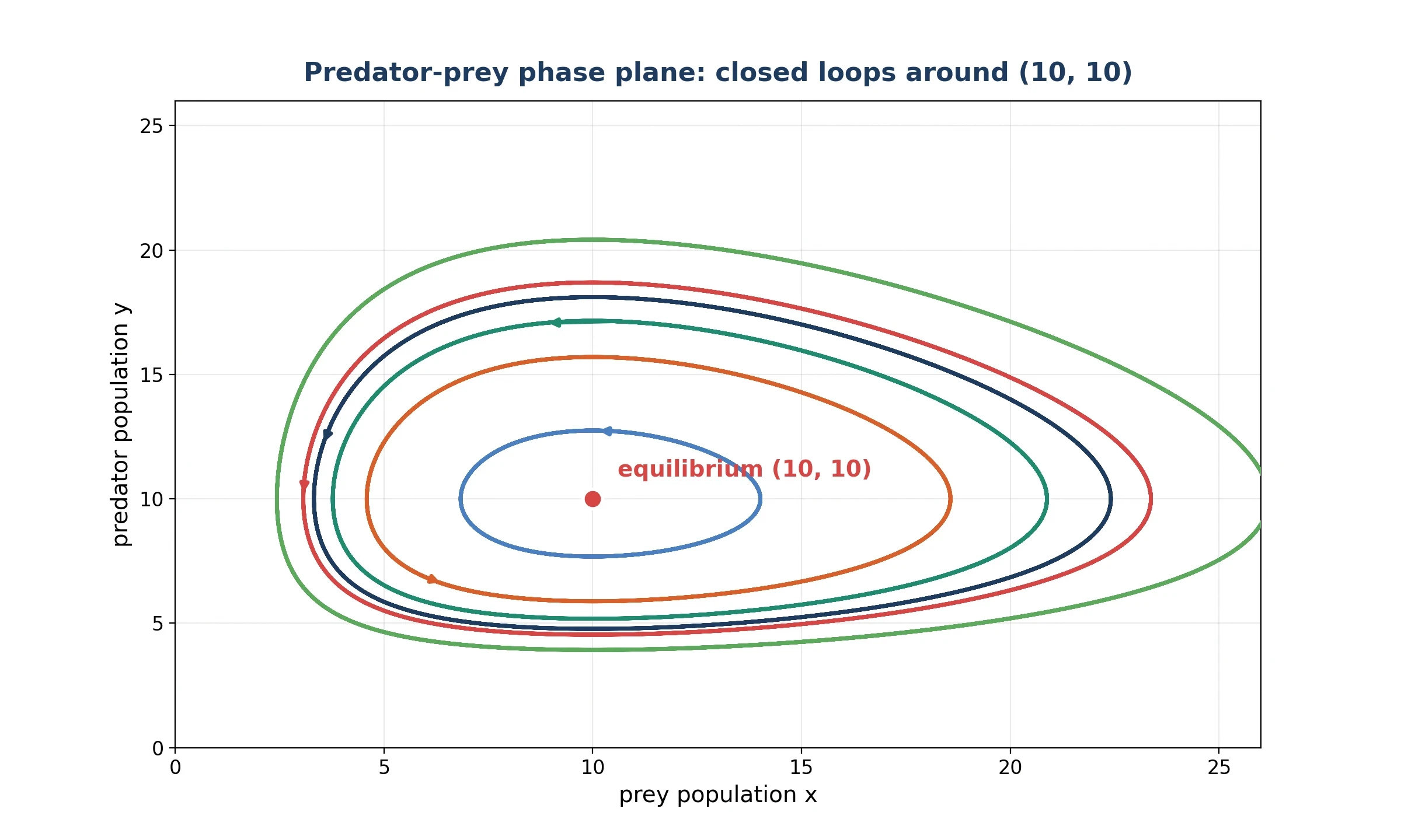
Small oscillations around the equilibrium have a period of about 8.89 time units, from 2 pi divided by the square root of alpha times gamma. The full nonlinear system keeps the cycles closed: the populations never settle and never run away, and the phase plane is a set of nested loops, each one a possible history chosen by the starting populations.
What the cycles do and do not prove
The closed loops in the phase plane are a mathematical fact about the model, and they are not a fact about the world. The model assumes prey grow exponentially without predators, predators die exponentially without prey, encounters are proportional to the product of the two populations, and there is no carrying capacity, no age structure, and no space. Real ecosystems violate every one of those assumptions, so the model is a starting point, not a forecast.
Kermack and McKendrick, 1927
William Ogilvy Kermack and Anderson Gray McKendrick published A Contribution to the Mathematical Theory of Epidemics in the Proceedings of the Royal Society A, volume 115, pages 700 to 721, in 1927, the paper having been received on 13 May 1927, from the Laboratory of the Royal College of Physicians in Edinburgh. It built on the work of Ross and Hudson from 1915 to 1917, and it was the first theory to account explicitly for the age of infection. The paper, and the two that followed in 1932 and 1933, were republished in the Bulletin of Mathematical Biology in 1991. The original 1927 model is a PDE model structured by age of infection; the familiar SIR equations are a special case of it, with a constant removal rate.
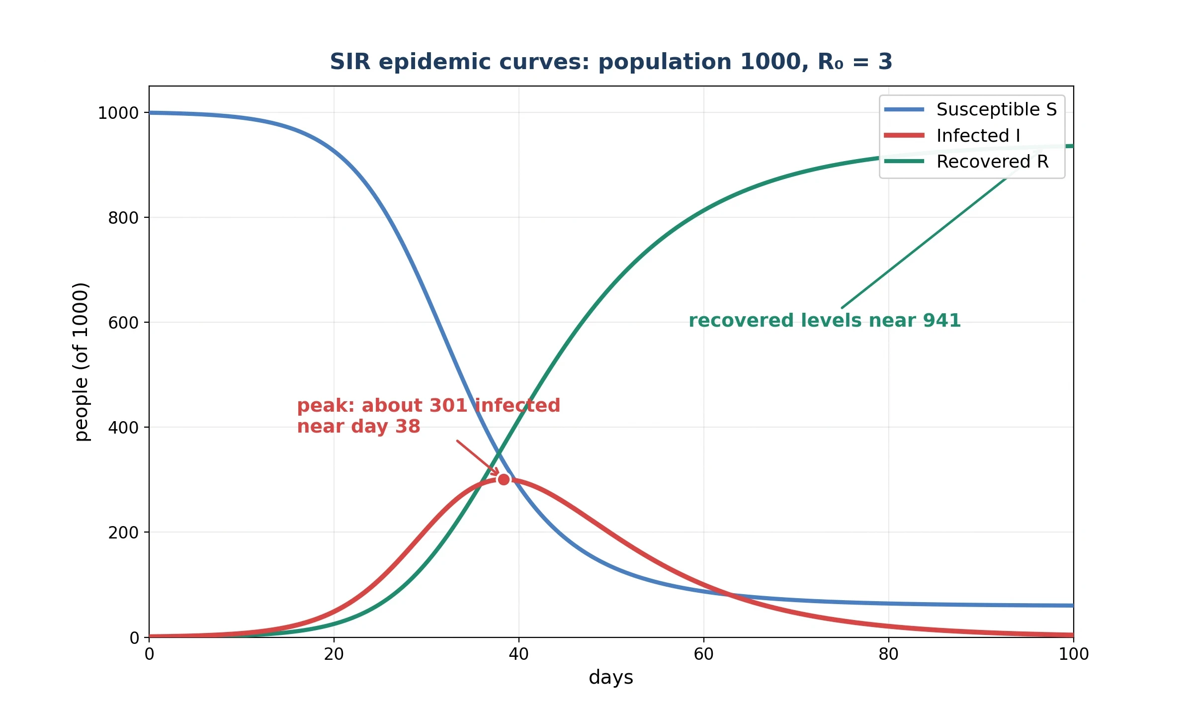
The SIR model divides a population into three groups: S for susceptible, I for infected, and R for recovered, and it writes a differential equation for each — three coupled differential equations that run the epidemic. The equations are dS/dt equals minus beta times S times I over N, dI/dt equals beta times S times I over N minus gamma times I, and dR/dt equals gamma times I, where N is the total population and beta and gamma are the transmission and recovery rates. The model is deterministic: the same starting values give the same curves, every time, and chance enters only when the model is extended, as our article on what probability is explains. The paper itself is available through the Royal Society, and the history of the 1927, 1932, and 1933 papers as a series is set out in the MacTutor account of epidemic theory.
R0 and the threshold, worked
The key number in the SIR model — one of the most used differential equations in public health — is R0, the basic reproduction number, equal to beta divided by gamma: the average number of new infections each infected person causes in a fully susceptible population. Take beta equal to 0.3 per day and gamma equal to 0.1 per day, in a population of 1000, starting with S0 equal to 999 and I0 equal to 1. Then R0 equals 3.0. An epidemic grows when the susceptible fraction exceeds 1 over R0, which is one third; here it starts at 0.999, far above one third, so the epidemic grows. The early growth rate is beta minus gamma, or 0.2 per day, and the early doubling time is the natural logarithm of 2 divided by 0.2, or 3.47 days.
A fine numerical integration gives the rest of the story: the infected curve peaks at about 301 near day 38, and the recovered curve levels off near 941 of the 1000 people. Both numbers are approximate, from numerical integration. The shape is the point, and the shape is robust: the infected rise, peak, and fall, the susceptible fall in an S-shape, and the recovered rise in an S-shape to a final level below the whole population, because the epidemic ends before everyone has been infected.
What SIR leaves out
The SIR model leaves out a great deal. There are no births and no deaths, so the population is fixed. There is no loss of immunity, so recovery is permanent — what immunity means in the body is the subject of our article on how vaccines work. Everyone mixes equally, so a hermit and a market trader have the same chance of meeting an infected person, which is false: real epidemics spread on contact networks, and the mathematics of those networks belongs in our article on graph theory. There is no age structure, no space, no variation in infectiousness, and no behaviour change as the epidemic grows. Real data also scatter around the model's curves — the spread of that scatter is the subject of our article on the normal distribution, while updating an estimate of R0 as new data arrive is the job of Bayes' theorem. The 1932 and 1933 papers extended the model to endemic disease and recurring epidemics.
I watched a case curve rise and fall once during an outbreak that filled the news, checking the numbers each morning and plotting them on the back of an envelope, and the shape that emerged was the SIR shape: a slow start, a steep climb, a peak, a fall, and a long tail. The numbers were real people, and the curve was a model, and the gap between them was the point. I kept the envelope. It taught me that a differential equation is not a prediction machine. It is a way of seeing the shape of a story while the story is still happening.
14. When There Is No Formula: Numerical Methods and Chaos
Euler's method, 1768
Euler's method is the simplest numerical method for differential equations there is, and it is also the oldest one-step method, published by Euler in 1768. The idea is disarmingly plain: follow the slope for one small step, then re-measure. At the starting point, the equation tells you the slope. Walk along that slope for a small step h, and you arrive at a new point, an approximation to the true solution, where the equation tells you a new slope. Repeat, and the points trace an approximate solution, a polygon that follows the true curve. The smaller the step, the closer the polygon hugs the curve, and the more steps the computation costs.
Euler against the exact answer, worked
Take dy/dx equals y, with y of 0 equal to 1, and compute y at x equal to 1, where the exact answer is e, which is 2.718282. With step 0.5, two steps, Euler gives 2.250000. The error is minus 0.468282, or minus 17.23 percent. With step 0.2, five steps, Euler gives 2.488320, an error of minus 0.229962, or minus 8.46 percent. With step 0.1, ten steps, Euler gives 2.593742, an error of minus 0.124539, or minus 4.58 percent. With step 0.05, twenty steps, Euler gives 2.653298, an error of minus 0.064984, or minus 2.39 percent. Each halving of the step roughly halves the error, and the answers climb toward the exact value from below, because the method follows the slope at the start of each step while the slope is growing.
Runge and Kutta, 1895 and 1901
Carl Runge published on the numerical solution of differential equations in 1895, in the Mathematische Annalen, volume 46, pages 167 to 178. Karl Heun introduced a third-order method in 1900. Wilhelm Kutta published his paper in 1901, in the Zeitschrift für Mathematik und Physik, volume 46, pages 435 to 453, taking the analysis to order 5 and producing the classic fourth-order Runge-Kutta method. The idea is to sample several slopes per step, not one — the slope at the start, the slope at the middle estimated from the start, the slope at the middle again, and the slope at the end — and take a weighted average of them as the slope for the step. The classic fourth-order method is fourth-order accurate: halving the step divides the error by sixteen, not by two, and that is why it is the workhorse of numerical differential equations.
Lorenz, 1963
Edward N. Lorenz, at MIT, published Deterministic Nonperiodic Flow in the Journal of the Atmospheric Sciences, volume 20, pages 130 to 141, in March 1963, the manuscript having been received on 18 November 1962 and revised on 7 January 1963. The paper reduced a model of convection — warm air rising, cool air sinking — to three coupled nonlinear ordinary differential equations, with the classic parameters sigma equal to 10, beta equal to 8 over 3, and rho equal to 28. The solutions were deterministic and nonperiodic: they never repeated, and they showed sensitive dependence on initial conditions, so two starting points a hair apart produced futures that diverged until they had nothing in common. The paper was rarely cited until about 1975, and from 1980 onward it has been cited on the order of 100 times per year.
The Lorenz system is the proof that deterministic does not mean predictable in practice. Three simple differential equations, no randomness anywhere, and a future that cannot be computed far ahead, because any tiny error in the starting values grows until it swallows the prediction. The full story — the butterfly effect, the strange attractor, the geometry of the divergence — belongs in our article on chaos theory, and the fractal shape of the attractor belongs in our article on fractals. The Lorenz equations are three ODEs: deterministic, and unpredictable over long times, and that combination is why numerical methods and chaos theory belong together.
Why computers changed the subject
Computers changed differential equations because most differential equations have no closed-form solution, and a computer can compute what a formula cannot give. Before computers, the solvable equations were the subject and the unsolvable ones were set aside. After computers, the unsolvable equations became the subject, and the solvable ones became the test cases that check the solvers. A numerical solution is a real solution: it is a table of values, or a curve drawn through them, that satisfies the equation to within a known error, and the error can be made as small as the computation allows. Those computations now run on machines linked across the world, and the network they use is explained in our article on how the internet works.
15. Common Misconceptions About Differential Equations
"A differential equation is just a hard algebra equation"
No. An algebra equation asks for a number, and its answer is a number. A differential equation asks for a function, and its answer is a curve: the unknown in dy/dx equals y is not a value of y, but the whole function y, at every x, and the equation is a condition the function must satisfy everywhere. Algebra finds points. Differential equations find curves.
"Every differential equation has a neat formula solution"
No. Most differential equations have no closed-form solution at all, and that is not a failure of the subject. It is a fact about the world: the equations that describe real systems are usually too tangled for a formula, and the solutions are computed, step by step, by the numerical methods of section 14. A numerical solution is a real solution, with a known error, and the Lorenz equations prove that a system can be perfectly deterministic and still have no formula. The logistic equation has a neat formula; the Lotka-Volterra equations do not, in elementary terms, and their cycles are studied through phase planes and computation. The formula is not the standard. The curve is.
"An initial condition is a detail"
No. An initial condition selects the solution. The same differential equation with a different starting value is a different story: a cup starting at 90 degrees and a cup starting at 60 degrees obey the same cooling rule, and their curves are different members of the same family. The slope field of section 5 shows it at a glance: one equation, many curves, and the starting point is the finger that points at one of them. The starting value is where the story begins, and the story depends on it.
"Nonlinear means unsolvable"
No. Nonlinear means no superposition and usually no formula, not no understanding. The Lotka-Volterra equations are nonlinear, and their cycles are understood completely through the phase plane: closed loops, an equilibrium at (10, 10), a period of about 8.89 for small oscillations. The logistic equation is nonlinear, and its S-curve is understood completely, with an exact formula. Nonlinear equations are studied with phase planes, numerical methods, and linearisation around equilibria. Unsolvable is a different word, and it belongs to equations that have no solution at all, not to equations that have no formula.
"A model that fits is a model that is true"
No. Malthus's model fits the early growth of a population and misses the limit. The logistic model fits the S-curve and misses the moving carrying capacity. The Lotka-Volterra model fits the cycles and misses the carrying capacity, the disease, and the weather. The SIR model fits the rise and fall of an epidemic and misses the networks, the behaviour change, and the births and deaths. Each model fits something and misses something, and the fit is not the test. The test is whether the model survives being checked against the world. A curve that fits the past and fails the future was never true. It was only fitting.
"Differential equations are only for physicists"
No. Populations, epidemics, circuits, ecology, and finance all run on differential equations, and the list grows every year. The cooling cup is a kitchen, a chemical plant, a body. The logistic curve is a population, a market, an epidemic. The SIR model is public health. The equations are a language, and a language belongs to everyone who has something changing to describe. The physicists were first, because Newton needed the language for motion, but the language has been borrowed by every science since.
16. What Change Leaves Behind
One language, many stories
Cooling coffee, a swinging spring, a growing population, a spreading epidemic: the same few equation shapes, different nouns. The first-order linear equation governs the coffee and the circuit, the second-order linear equation governs the spring and the pendulum, the logistic equation governs the population, the SIR equations govern the epidemic, the heat equation governs the rod, and the wave equation governs the string. Learn the shapes of differential equations, and the world starts to repeat itself in a helpful way: a new phenomenon arrives, and the first question is which shape it wears, the second what the constants are, and the third whether the shape fits.
The pattern of the article in one paragraph
Classify first, and let the classification choose the method. Check existence, and ask whether the solution is unique before you trust it. Try separation of variables for equations that pull apart, integrating factors for linear first-order equations, and the characteristic equation for second-order linear equations with constant coefficients. When no formula exists, compute. Always check the model against the world, and remember what the model leaves out. That is the pattern of differential equations: a small set of moves, applied with care, to a large set of changing things.
Try it yourself
Three exercises, in order of difficulty, each one a real piece of the subject.
- Sketch a slope field for dy/dx equals y, and draw the curves through (0, 1) and (0, 2), following the segments. Check that both look like exponentials, one higher than the other.
- Compute a cooling time for a drink, using the numbers in section 11: a drink at 80 degrees in a 20-degree room, with k equal to 0.1 per minute, reaches 30 degrees after how long? Work it out from the solution T of t equals 20 plus 60 times e to the power minus 0.1 t, and compare your answer with the 19.46 minutes for the 90-degree cup.
- Find the equilibrium of a predator-prey pair with the worked parameters of section 13: alpha equal to 1.0, beta equal to 0.1, delta equal to 0.05, gamma equal to 0.5. Set both rates of change to zero, solve for x star and y star, and check that you get (10, 10). Then ask what happens to the equilibrium if gamma doubles.
Frequently Asked Questions
What is a differential equation?
A differential equation is an equation that links a function to its derivatives, and solving it means finding the function. It says how fast something changes, in terms of where it is now, and its answer is a curve, not a number — a cup cooling, a population growing, a spring swinging. The equation is the rule about the rate; the solution is the story of the change.
What is the difference between ODEs and PDEs?
An ordinary differential equation involves a function of one variable and ordinary derivatives, while a partial differential equation involves a function of several variables and partial derivatives. A cooling cup is an ODE, because its temperature depends on time alone; a cooling metal bar is a PDE, because its temperature depends on position and time together. ODEs describe a single unfolding story, and PDEs describe a field spread over space and time, as section 3 explains.
How do differential equations model the real world?
Write the rate of change as a rule, solve the equation or compute the solution, and check the answer against measurements: a cooling cup follows Newton's law of cooling, a population follows exponential growth and then the logistic equation, a circuit follows the RC equation, and an epidemic follows the SIR model. Each model is a set of differential equations with constants fitted to the world, and each is checked by whether its curves match the measurements, as sections 9 to 13 show.
What is Newton's second law as a differential equation?
Newton's second law says force equals mass times acceleration, and acceleration is the second derivative of position with respect to time, so the law is m times d squared x over dt squared equals F. For a spring, the force is minus k times x, giving a second-order equation whose solution is simple harmonic motion; for a pendulum of length 1 metre, the period is 2.006 seconds, as section 9 shows.
How do you solve a differential equation?
There is no single method for solving differential equations. Separation of variables works when the x and y parts pull apart, as in section 6. Integrating factors solve linear first-order equations (section 7), the characteristic equation solves second-order linear equations with constant coefficients (section 8), and when no formula exists, numerical methods compute the solution (section 14). The classification of section 4 chooses the method.
What is the logistic growth equation?
The logistic growth equation is dN/dt equals r times N times one minus N over K, where r is the growth rate and K is the carrying capacity. Verhulst published it in 1838, and its solution is the S-curve: N of t equals K divided by one plus A times e to the power minus r t. With K equal to 1000, a starting population of 100, and r equal to 0.5, the population reaches 500 at time 4.39 and 942.83 at time 10, as section 10 shows.
What is the SIR model?
The SIR model divides a population into susceptible, infected, and recovered groups, and writes a differential equation for each. Kermack and McKendrick published it in 1927. Its key number is R0, equal to beta divided by gamma, and an epidemic grows when the susceptible fraction exceeds 1 over R0. With R0 equal to 3, the infected peak at about 301 near day 38 in the worked example, approximately, as section 13 shows.
Can every differential equation be solved exactly?
No. Most differential equations cannot be solved exactly, in the sense of a formula in elementary terms, and that is why numerical methods exist. Euler's method follows the slope step by step, and the Runge-Kutta method samples several slopes per step for far greater accuracy. The Lorenz equations of 1963 are three simple ordinary differential equations with no closed-form solution, deterministic yet unpredictable over long times, as section 14 explains.
Sources
- LibreTexts, "0.3: Classification of Differential Equations" (Lebl, Differential Equations for Engineers). ODE versus PDE, order, linearity, homogeneity, and autonomous equations. https://math.libretexts.org/Bookshelves/Differential_Equations/Differential_Equations_for_Engineers_(Lebl)/0%3A_Introduction/0.3%3A_Classification_of_Differential_Equations
- Parker, "Who Solved the Bernoulli Differential Equation and How Did They Do It?", College Mathematics Journal, volume 44, number 2 (2013). Bernoulli equation proposed December 1695; Leibniz 1696; Johann Bernoulli's method. https://old.maa.org/sites/default/files/pdf/upload_library/2/Parker-CMJ-2014.pdf
- "Differential Equations: A Historical Refresher", arXiv:2012.06938 (2020). Leibniz 11 November 1675; Newton Methodus fluxionum 1671, published 1736; Bernoulli 1690 separation of variables; integrating factors. https://arxiv.org/pdf/2012.06938
- MAA Convergence, Cummings and Parker, "D'Alembert, Lagrange, and Reduction of Order — Enter Euler" (September 2015). Euler 1739 correspondence; 1743 paper on constant-coefficient equations; Lagrange 1774-1775. https://old.maa.org/node/665681
- MacTutor History of Mathematics, University of St Andrews, "Epidemic theory" (Kermack-McKendrick). The 1927 paper reference; the 1927, 1932, 1933 series; the threshold theorem. http://mathshistory.st-andrews.ac.uk/Extras/Epidemic_theory/
- PMC, "Alfred J. Lotka and the origins of theoretical population ecology" (2015). Lotka 1920 PNAS paper; Elements of Physical Biology 1925; Volterra independently 1925-1926. https://pmc.ncbi.nlm.nih.gov/articles/PMC4534218/
- Brown University, "Biography of Joseph Fourier" (Mathematica Tutorial). Fourier memoir 1807; Theorie analytique de la chaleur 1822; the "profound study of nature" quotation. https://www.cfm.brown.edu/people/dobrush/am34/Mathematica/ch5/joseph.html
- Encyclopedia of Mathematics, "Pearl-Verhulst logistic process". Verhulst 1838, pages 113-121; Pearl and Reed 1920; Lotka 1925. https://encyclopediaofmath.org/wiki/Pearl%E2%80%93Verhulst_logistic_process
- Boston University, Lorenz 1963 paper PDF, "Deterministic Nonperiodic Flow". Manuscript received 18 November 1962; Journal of the Atmospheric Sciences, volume 20, pages 130-141, March 1963. https://math.bu.edu/people/mabeck/Fall14/Lorenz63.pdf
- Wikipedia, "Newton's law of cooling". Published anonymously 1701, "Scala graduum Caloris", Philosophical Transactions, volume 22, pages 824-829; Dulong and Petit 1817. https://en.wikipedia.org/wiki/Newton%27s_law_of_cooling
- Wikipedia, "Schrödinger equation". Postulated 1925, published 1926; Nobel Prize 1933; quantum counterpart of Newton's second law. https://en.wikipedia.org/wiki/Schr%C3%B6dinger_equation
- Wikipedia, "Malthusian growth model". Malthus, An Essay on the Principle of Population (1798); doubling about every 25 years. https://en.wikipedia.org/wiki/Malthusian_growth_model
- Wikipedia, "One-step method". Euler method published 1768; Runge 1895; Heun 1900; Kutta 1901. https://en.wikipedia.org/wiki/One-step_method
- Butcher, "A history of Runge-Kutta methods", Applied Numerical Mathematics, volume 20 (1996), pages 247-260. Runge 1895; Heun 1900; Kutta 1901. https://tlakoba.w3.uvm.edu/math6737/paper_1996_Butcher_RKhistory.pdf
- Fourier, Joseph, Theorie analytique de la chaleur, Paris: Firmin Didot Pere et Fils, 1822. English translation: The Analytical Theory of Heat, translated by Alexander Freeman, Cambridge University Press, 1878. The heat equation and Fourier series; the blockquote source, chapter 1, page 7. No URL invented for the book itself; the biography is Source 7.
- Newton, Isaac, Philosophiae Naturalis Principia Mathematica, London, 1687 (first edition 5 July 1687; second edition 1713; third edition 1726). Three laws of motion and universal gravitation. https://cudl.lib.cam.ac.uk/view/MS-ADD-03965
- Boyce, William E., DiPrima, Richard C., and Meade, Douglas B., Elementary Differential Equations and Boundary Value Problems, 12th edition, Wiley, 2021. Standard first-course text; historical notes on Euler, Lagrange and Laplace.
- Strogatz, Steven H., Nonlinear Dynamics and Chaos, 2nd edition, CRC Press, 2019. Lotka-Volterra phase planes, Lorenz system, numerical methods.
- Volterra, Vito, "Fluctuations in the Abundance of a Species considered Mathematically", Nature, volume 118, pages 558-560 (1926). DOI: 10.1038/118558a0.
- Kermack, William Ogilvy, and McKendrick, Anderson Gray, "A contribution to the mathematical theory of epidemics", Proceedings of the Royal Society of London, Series A, volume 115, number 772, pages 700-721 (1927). DOI: 10.1098/rspa.1927.0118.
- Lorenz, Edward N., "Deterministic Nonperiodic Flow", Journal of the Atmospheric Sciences, volume 20, pages 130-141 (1963). DOI: 10.1175/1520-0469(1963)020<0130:DNF>2.0.CO;2.
- Newton, Isaac, "Scala graduum Caloris. Calorum Descriptiones and signa", Philosophical Transactions of the Royal Society of London, volume 22, number 270, pages 824-829 (1701). DOI: 10.1098/rstl.1700.0082.
- Lotka, Alfred J., "Analytical note on certain rhythmic relations in organic systems", Proceedings of the National Academy of Sciences USA, volume 6, number 7, pages 410-415 (1920). DOI: 10.1073/pnas.6.7.410.
- Picard, Emile, "Memoire sur la theorie des equations differentielles", Journal de l'Ecole Polytechnique, volume 60, pages 137-204 (1890); and Lindelöf, Ernst, "Sur l'application de la methode des approximations successives aux equations differentielles ordinaires du premier ordre", Comptes Rendus Hebdomadaires des Seances de l'Academie des Sciences, volume 118, pages 454-457 (1894). The two papers behind the Picard-Lindelöf theorem; journal citations as given in standard references, no DOI listed.
- MacTutor History of Mathematics, University of St Andrews, "Jean d'Alembert (1717–1783)". Pioneer in the study of partial differential equations; the 1747 vibrating-strings paper contains the first appearance of the wave equation in print. https://mathshistory.st-andrews.ac.uk/Biographies/DAlembert/
- Imperial College London, "History of Mathematics" lecture notes, week 8. Laplace's equation (1782/85, 1787/89); Théorie des attractions des spheroides et de la figure des planètes (1782). https://www.ma.imperial.ac.uk/~bin06/HoM/m3hw8.pdf
- Schrödinger, Erwin, "Quantisierung als Eigenwertproblem", Annalen der Physik, volume 79 (1926), pages 361–376. DOI: 10.1002/andp.19263840404.