
1. The Shape That Broke Geometry
A coastline with no length
Take a map of Britain and a ruler, and measure the coastline. Now take a shorter ruler and measure it again. The second answer will be longer. Take a still shorter ruler and the coastline grows again. There is no point at which the number settles down. Every shorter ruler finds more bays, more inlets, more wiggles that the longer ruler skipped over, and the total keeps climbing.
This is not a trick of bad measuring. It is a real property of the coastline itself. A straight line has a length that every ruler agrees on. A coastline does not. The question "how long is the coast of Britain?" turns out to have no single answer, only an answer that depends on the size of the ruler you use. That discovery, made in the middle of the twentieth century and explained by Benoît Mandelbrot in 1967, opened a door into a whole geometry that the textbooks had left out. The shapes inside that geometry are called fractals, and this article is about them.
I first met the coastline problem the slow way, on a wet afternoon with a paper map, a piece of string, and a ruler. I was trying to measure a stretch of coast for a school project, and the string kept coming out longer every time I was more careful. I blamed the string. Then I blamed my hands. It took me years to learn that the coast itself was the problem — or rather, that my idea of length was too narrow for the coast. That afternoon stayed with me because it was the first time a simple measurement refused to behave, and the refusal turned out to be the interesting part.
The puzzle is sharper than it first looks. Spain and Portugal once disagreed by roughly twenty percent about the length of their shared border, not because either side was lying or careless, but because each side measured with a different ruler length. The English meteorologist Lewis Fry Richardson noticed this in the 1920s and 1940s: the shorter the ruler, the longer the measured border. He wrote the pattern down as a law, and it sat there, unexplained, for decades. Mandelbrot saw what it meant. A coastline behaves like a shape that has detail at every scale, and a shape like that cannot be measured the way a smooth curve can.
What this article will show you
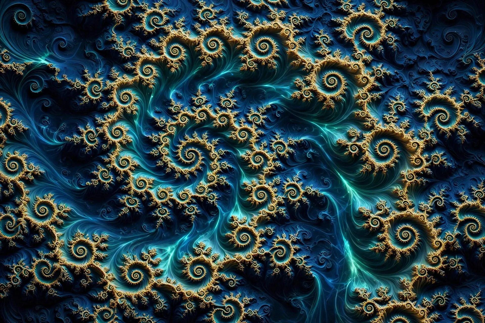
Fractals are patterns that repeat themselves at different scales. A small piece of a fractal looks like the whole thing, or nearly like it, or at least like it in its statistics. That one idea — the same pattern, again and again, smaller and smaller — builds the Koch snowflake, the Sierpinski triangle, the branching of trees and lungs, and the most famous picture in all of mathematics, the Mandelbrot set.
We will build the classic fractals step by step, with the numbers worked out in full, so you can check every claim yourself. We will see how a snowflake can have an infinite perimeter and a finite area at the same time, and why that is not a contradiction. We will learn how to measure roughness with a number called fractal dimension, a number that is allowed to be a fraction. We will meet the Mandelbrot set, a shape generated by one tiny rule, and its cousins, the Julia sets. We will look at where fractals really appear in nature — and where they do not — and finish with what fractals are actually good for, from phone antennas to financial markets, plus the myths that need clearing away.
You do not need much mathematics to follow along. A little school algebra helps, and the one place where we need complex numbers, I will explain them in a single paragraph and point you to the full treatment in our article on imaginary numbers. Everything else is built from scratch, one step at a time.
2. What Is a Fractal?
Self-similarity: the part that looks like the whole
The defining idea of a fractal is self-similarity. Take a piece of the shape, magnify it, and you see something that looks like the whole shape again. Magnify a piece of that piece, and there it is again. The pattern repeats across scales.
Self-similarity comes in three strengths. Exact self-similarity means a magnified part is an identical copy of the whole. The Koch curve and the Sierpinski triangle do this: zoom in on any corner and you find the same shape, perfectly. Only mathematical fractals, built by exact rules, manage this. Approximate self-similarity means parts resemble the whole but with variation. A fern is the classic case: each leaflet looks like a small frond, but no two leaflets are identical. Statistical self-similarity is looser still: no two stretches match, but the statistics repeat — the roughness, the distribution of wiggles, the way the pattern varies. Coastlines work this way, and so do clouds and price charts. Mandelbrot introduced this statistical version in his 1967 coastline paper, writing that each portion of a coastline can, in a statistical sense, be considered a reduced-scale image of the whole.
Detail at every scale
A second property goes with self-similarity: detail at every scale. A circle looks smooth no matter how closely you look. Zoom in on a circle and it just looks like a straighter and straighter line. A fractal does the opposite. Zoom in and new structure appears. Zoom in again and more structure appears. In a mathematical fractal, this never stops. There is no smallest scale at which the shape finally becomes smooth.
This is why the coastline resists measurement. A ruler of one kilometre skips the bays. A ruler of one hundred metres finds them. A ruler of one metre finds the rocks inside the bays. A ruler of one centimetre finds the grains of sand. Each scale adds length, and for a mathematical fractal the process has no end. For a real coastline it does end — at atoms, eventually — but it goes on far longer than our everyday intuition expects, from hundreds of kilometres down to metres, and that is enough to make the measured length depend on the ruler.
A dimension that is not a whole number
The third property is the strangest. A fractal has a dimension that is not a whole number. We are used to dimensions being 1, 2, or 3: a line is one-dimensional, a square is two-dimensional, a cube is three-dimensional. A fractal can sit in between. The Koch curve has dimension about 1.26. The Sierpinski triangle has dimension about 1.59. These numbers are not metaphors. They are measured quantities, and Section 7 will show you exactly how to compute them.
Mandelbrot's own definition, the one he gave in his writing on the subject, was this: a fractal is a set whose Hausdorff dimension strictly exceeds its topological dimension. In plain words, a shape that is rougher than the whole-number dimension it lives in. A curve, topologically speaking, is one-dimensional. If its Hausdorff dimension is 1.26, it is rougher than a curve and smoother than a surface, and that roughness is real and measurable. The MacTutor history of fractal geometry gives the full background on how this definition grew out of work that began decades before Mandelbrot named the field.
3. A Word Invented in 1975
Benoît Mandelbrot and the Latin fractus
Benoît Mandelbrot was born in Warsaw in 1924, grew up in France, and spent much of his career at IBM, where he had access to computers powerful enough to draw pictures no one had ever seen. He was a restless thinker who moved between mathematics, economics, and the study of nature, and he kept noticing the same rough, irregular shapes turning up in places where the textbooks said smooth shapes should be. Coastlines, clouds, price charts, the branching of trees: none of them looked like the circles and triangles of school geometry.
In 1975 he gave these shapes a name. He coined the word fractal from the Latin fractus, meaning broken or fractured. The word was a good choice. It says the shape is irregular, fragmented, rough — broken in the sense that it refuses to be smooth. It also says, quietly, that the roughness is the point, not a defect.
Three books: 1975, 1977, 1982 — what each one did
Mandelbrot published the word in a French book, Les Objets Fractals: Forme, Hasard et Dimension, in 1975. Two years later, in 1977, an English translation appeared under the title Fractals: Form, Chance and Dimension. That 1977 volume is a translation, not a new book — a distinction worth making, because it is often misdescribed. Then in 1982 came the revised and enlarged book that made the subject famous, The Fractal Geometry of Nature. That is the book whose first page carries the most quoted sentence in the whole field, the sentence we will meet at the end of Section 10.
The three dates tell a story about how an idea spreads. In 1975 the word existed, mostly in French, mostly among specialists. In 1977 it became available in English. In 1982 it arrived as a full argument, with pictures, that the geometry of nature is fractal geometry — that clouds, mountains, coastlines, and trees belong to a geometry of roughness, not the smooth geometry of Euclid. The pictures mattered as much as the words. Computers could finally draw these shapes, and once people saw them, the idea was impossible to unsee.
Why nobody had a word for this before
It is worth asking why something so common took so long to get a name. Part of the answer is that mathematicians had seen these shapes before — and had dismissed them. Weierstrass's curve with no tangent, Cantor's dust, Peano's space-filling curve: all of them were known by the early twentieth century, and all of them were treated as curiosities, even as monsters. They were the exceptions that proved the rule that good curves are smooth. Nobody had put them together into a single family with a single name and a single way of measuring them.
4. The Monsters Before Mandelbrot
Weierstrass's curve with no tangent (1872)
In 1872, Karl Weierstrass presented a function to the Berlin Academy that shocked his audience. It was a curve that is continuous everywhere but has no tangent anywhere. Picture a curve so jagged that, no matter how closely you zoom in, it never straightens out into a smooth line. At every point, the slope is undefined. There is no place on the curve where you can draw a tangent and say "this is the direction the curve is going here."
Weierstrass's construction used an infinite sum of wiggly cosine waves, each one smaller and faster than the last. The result is a curve that is, in a real sense, all corners. It was the first mathematical monster: a shape that obeyed the rules of analysis and violated every intuition about what a curve should look like. Mathematicians of the time were so disturbed that the curve was described as a monster, a pathological case, something to be fenced off from respectable mathematics.
Cantor's dust (1883) and Peano's space-filling curve (1890)
Georg Cantor, in 1883, published a construction that is now called the Cantor set, or Cantor's dust. Start with a line segment. Remove the middle third. Remove the middle third of each remaining piece. Keep going forever. What is left? Infinitely many points, but no intervals at all — a dust of points with total length zero, yet uncountably infinite in number. Its fractal dimension, computed the way Section 7 will show, is about 0.6309: less than 1, because it is sparser than a line, but more than 0, because it is far richer than a scatter of isolated points.
Seven years later, in 1890, Giuseppe Peano published a curve that fills a square. A curve, one-dimensional by any ordinary reckoning, that passes through every point of a two-dimensional region. It was another monster, another violation of the idea that dimension is a fixed, obvious property of a shape. A curve could be two-dimensional, in effect. The ground was shifting under the whole idea of dimension, and it would take Hausdorff's work in 1918 to give the shift a firm footing.
Why mathematicians called them monsters — and ignored them
These shapes were called monsters because they broke the bargain that mathematics had made with intuition. The bargain was that curves are smooth, that dimension is a whole number, that length is a well-defined property of a curve. Each monster broke one part of the bargain, and the field's response was to label them pathological — interesting, perhaps, but not representative of anything real.
The next two sections take up the two friendliest monsters — the ones you can build yourself with a pencil and a ruler. The Koch snowflake and the Sierpinski triangle are the gateway fractals, and they carry the whole subject in miniature: a simple rule, repeated forever, producing a shape with properties that seem impossible until you do the arithmetic.
5. The Koch Snowflake: Infinite Edge, Finite Area
The rule: cut the middle third, add a tent
Helge von Koch was a Swedish mathematician who, in 1904, published a curve that did what Weierstrass's curve did, but with a construction so simple that anyone can follow it. He wanted a continuous curve with no tangent anywhere, and he wanted it built from plain geometry rather than an infinite sum of waves. His paper, "Sur une courbe continue sans tangente, obtenue par une construction géométrique élémentaire", appeared in Arkiv för Matematik, volume 1, pages 681 to 704. The snowflake is three Koch curves joined around an equilateral triangle.
The rule is this. Start with an equilateral triangle. Take each straight edge and divide it into three equal parts. Remove the middle third. Replace it with the two other sides of a small equilateral triangle built outward on that middle third — a little tent sticking out. That is one iteration. Now do the same thing to every new edge, and then to every edge after that, forever.
Worked example: the perimeter multiplies by 4/3 every time
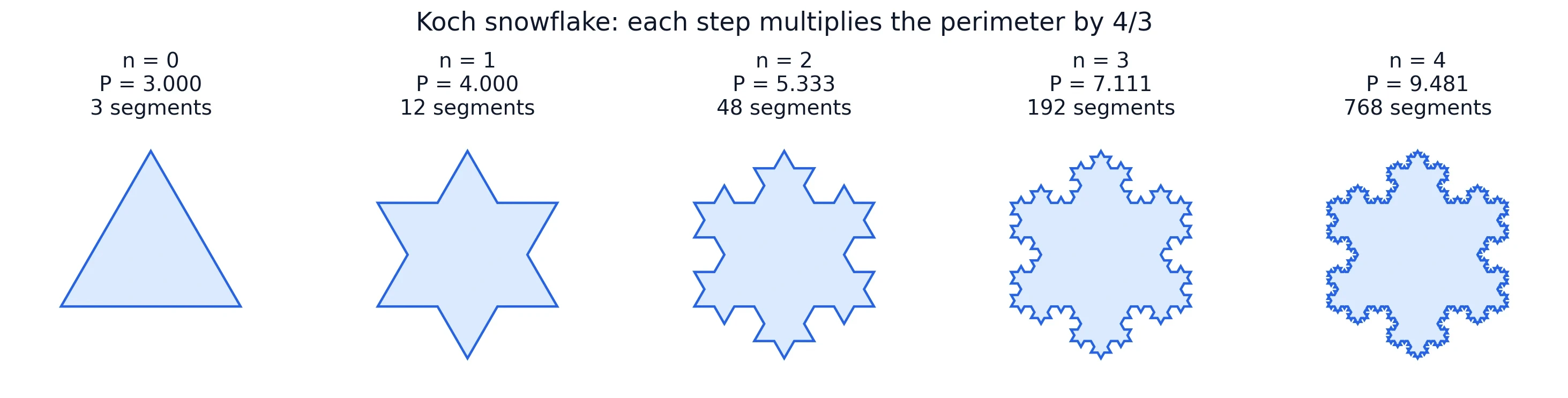
Here is the arithmetic, and it is worth doing slowly because the conclusion is startling. Each iteration replaces one segment of length L with four segments, each of length L divided by 3. So the total length of that piece grows by a factor of 4 divided by 3. Every iteration multiplies the whole perimeter by 4/3, exactly.
Start with a triangle whose sides are length 1, so the starting perimeter is 3. I recomputed the following numbers in Python, and you can check them with a calculator:
| Iteration n | Segments (3 × 4^n) | Perimeter (3 × (4/3)^n) | Area as fraction of starting triangle |
|---|---|---|---|
| 0 | 3 | 3.000000 | 1.000000 |
| 1 | 12 | 4.000000 | 1.333333 |
| 2 | 48 | 5.333333 | 1.481481 |
| 3 | 192 | 7.111111 | 1.547325 |
| 4 | 768 | 9.481481 | 1.576589 |
| 5 | 3,072 | 12.641975 | 1.589595 |
| 6 | 12,288 | 16.855967 | 1.595376 |
| 10 | 3,145,728 | 53.273180 | 1.599820 |
| Limit (n → infinity) | Infinite | Infinite | 1.600000 (8/5) |
The pattern is exact: perimeter after n iterations is 3 times (4/3) to the power n. At n = 10 the perimeter is already more than 53, from a starting perimeter of 3. At n = 20 it would be over 940. There is no ceiling. In the limit, the perimeter is infinite. A finite shape, drawn inside a page, with an edge longer than any number you can name.
Notice also the segment count: 3 times 4 to the power n. At n = 7 there are 49,152 segments. At n = 10 there are more than three million. This is why the snowflake defeats hand-drawing so quickly, and why computers were needed to see fractals properly.
Worked example: the area converges to 8/5 of the starting triangle
Now the other half of the paradox. While the perimeter explodes, the area settles down. Each iteration adds new triangles, but each round of additions is smaller than the last. The total area added in one iteration is 4/9 of the area added in the previous iteration, so the additions form a convergent geometric series — the same kind of series that appears whenever a quantity shrinks by a fixed fraction at each step, and whose sum is finite. If you want the full limit argument, our article on how calculus works walks through convergent series and limits in detail.
The numbers tell the story. After the first iteration the area is 4/3 of the starting triangle, about 1.333. After the second it is about 1.481. After the third, about 1.547. After the sixth, about 1.595. The growth slows with every step, and the total creeps toward a limit of 8/5 of the starting triangle — 1.6 times the original area, and no more. For a starting triangle of side 1, whose area is the square root of 3 divided by 4, about 0.433, the limit area is about 0.693. Finite, pinned down, and small.
The formula is: area after n iterations equals the starting area times 1 plus (3/5) times (1 minus (4/9) to the power n). As n grows, (4/9) to the power n shrinks to zero, and the bracket settles at 1 plus 3/5, which is 8/5. The snowflake's area is bounded forever by that number. It never reaches beyond it, no matter how many iterations you run.
Why the paradox is not a contradiction
Infinite perimeter, finite area. It sounds impossible, and the first time I worked through the numbers I checked them twice, convinced I had made an arithmetic error somewhere. I had not. The paradox dissolves once you see what "perimeter" is measuring here.
Perimeter measures length along a path that gets rougher at every scale. Each new generation of tiny tents adds length, and the additions never stop. But each new generation is also much smaller than the last, so the new tents fit inside a smaller and smaller fringe around the shape. Length can grow without bound while the region the shape occupies stays bounded, because length and area measure different things. Length counts the wiggliness of the boundary. Area counts the region enclosed. A boundary can wiggle without limit inside a bounded region, the way a coastline can keep adding bays inside the same stretch of coast.
The key is that the snowflake is not a smooth curve with a length in the ordinary sense. Its boundary is a fractal curve with dimension about 1.26 — rougher than a line, smoother than a surface — and the ordinary idea of length, which assumes a curve eventually straightens out when you zoom in, simply does not apply. The Koch snowflake is the cleanest demonstration in mathematics that "how long" can be a bad question for a rough shape. The same lesson, applied to a real coastline, is the subject of Section 8. And the idea that infinity can live inside a finite space is one our article on what infinity is explores from the other direction — here the infinite thing is a length, and the finite thing is an area.
6. The Sierpinski Triangle: The Shape That Deletes Itself
The rule: remove the middle, keep the corners
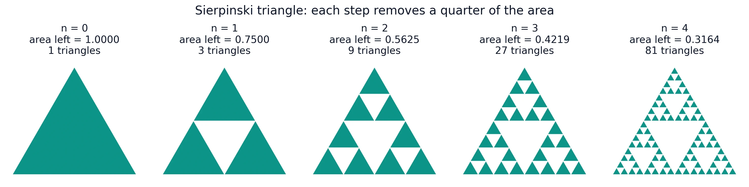
If the Koch snowflake builds by adding, the Sierpinski triangle builds by deleting. Wacław Sierpiński, a Polish mathematician, described it in 1915. Start with a solid equilateral triangle. Join the midpoints of its sides, which divides it into four smaller triangles, and remove the central one — the upside-down triangle in the middle, one quarter of the area. Three triangles remain, one at each corner. Now do the same to each of those three: remove the middle quarter of each. Keep going forever.
The result is a triangle full of holes, holes within holes, a lacework that never finishes. At each step the shape gets emptier, and yet it never disappears. Infinitely many points survive, arranged in a pattern that is exactly self-similar: each corner triangle is a half-size copy of the whole, and each of those contains three smaller copies, and so on without end.
Worked example: a quarter of the area gone at every step — area tends to zero
The arithmetic here is the mirror image of the Koch snowflake. Each iteration keeps 3/4 of the area that remained after the previous one. So the remaining area after n iterations is (3/4) to the power n. I recomputed these values in Python:
- After 1 iteration: 0.75 remains, 25 percent removed.
- After 2 iterations: 0.5625 remains, 43.75 percent removed.
- After 3 iterations: 0.421875 remains.
- After 4 iterations: 0.316406 remains.
- After 5 iterations: 0.237305 remains.
- After 10 iterations: 0.056314 remains — more than 94 percent of the area gone.
The limit is zero. The Sierpinski triangle, carried to infinity, has zero area. And yet it is not empty. It contains infinitely many points — the corners, the edges of the surviving triangles, and uncountably many more besides. A shape with no area and infinitely many points is strange, but it is not a contradiction. Area measures how much two-dimensional space a shape covers, and the Sierpinski triangle covers none of it in the limit, because every patch of it, however small, has a hole punched in it eventually. The points that survive are arranged along lines and corners, and the shape's dimension, about 1.585, sits between a line and a surface — which is exactly what you would expect for something too substantial to be a mere curve and too sparse to be a surface.
The smallest triangles tell the same story from the other side. After n iterations there are 3 to the power n of them, each with side length (1/2) to the power n of the original. After 5 iterations there are 243 triangles, each with side 1/32 of the original. The number of pieces grows, each piece shrinks, and the total area drains away.
Three ways to build the same triangle (removal, shrink-and-copy, chaos game)
One of the most satisfying facts about the Sierpinski triangle is that three completely different procedures produce exactly the same shape. The first is the removal construction we have just used: cut out the middle, repeat.
The second is shrink-and-copy. Take the whole triangle, shrink it to half size, and place three copies at the three corners. That gives you the shape after one iteration. Now take that shape, shrink it to half size, and place three copies at the corners again. Repeat forever. Same result, built by copying instead of deleting.
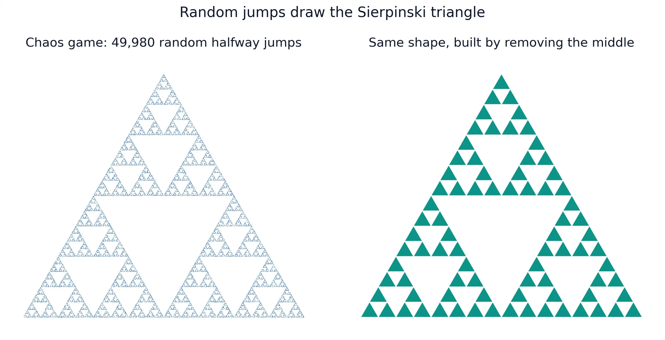
The third is the chaos game, and it is the most surprising of the three. Pick a random corner of the triangle. Start at any point. Jump halfway toward the chosen corner and mark a dot. Pick another random corner, jump halfway toward it, mark a dot. Repeat thousands of times. The dots do not scatter randomly across the triangle. They settle, with eerie precision, onto the Sierpinski triangle — the same lacework the removal rule produces. Randomness draws exact order. I first ran this on a sheet of graph paper with a die to choose corners, and after fifty dots the pattern was already visible, which felt like a small conjuring trick. It is not a trick. Each jump halves the distance to a corner, and the points that can be reached by such jumps are exactly the points of the Sierpinski triangle. The chaos game will return in Section 12, where it becomes a general method for drawing fractals.
The carpet and the sponge: the same idea in a square and a cube
The same idea works in other shapes. The Sierpinski carpet starts with a solid square, divides it into nine equal smaller squares, and removes the centre one. Repeat on each of the eight remaining squares. Eight copies at one-third scale give a dimension of log 8 divided by log 3, about 1.8928 — closer to 2 than the triangle, because the carpet keeps more of its area at each step.
The Menger sponge, described by Karl Menger in 1926, is the three-dimensional version. Start with a cube, divide it into twenty-seven smaller cubes, and remove the centre cube of each face plus the cube at the very centre — seven cubes removed, twenty kept. Repeat forever. The result has dimension log 20 divided by log 3, about 2.7268: a shape that is mostly holes, yet still connected, with infinite surface area and zero volume. It is a sponge in the most literal mathematical sense.
And the ancestor of them all, Cantor's dust from Section 4, is the one-dimensional version: remove the middle third of a line, repeat. Its dimension is log 2 divided by log 3, about 0.6309 — below 1, because it is sparser than a line. Together these four shapes show that the removal idea scales across dimensions, and that fractal dimension is the number that keeps track of how much survives each round of cutting.
7. Fractal Dimension: Measuring Roughness
Why whole-number dimensions fail
Dimension feels like a settled question. A line is one-dimensional, a plane is two-dimensional, a solid is three-dimensional, and that is that. The Koch curve breaks this settlement. It is a curve, so it ought to be one-dimensional. But it is far too rough to be an ordinary curve: it fills space more thoroughly than a line, winding and branching into every corner of its region. It is not a surface either; it has no area. It sits in between, and the whole-number system has no name for where it sits.
The problem is not with the curve. The problem is with the measuring tool. Whole-number dimension counts directions: how many independent directions can you move in? A line has one, a plane has two, a solid has three. But roughness is a different kind of quantity. A rough curve explores its space more thoroughly than a smooth one, and the right question is not "how many directions?" but "how much more of the shape appears when you magnify it?" Fractal dimension answers that question, and it answers with a fraction.
The copy-and-scale test: D = log N / log S
The test is simple enough to run on any exactly self-similar shape. Magnify the shape by a scale factor S, and count how many copies N of the original you need to build the magnified version. For ordinary shapes the relation is N equals S to the power D, where D is the dimension. A line segment magnified by 2 needs 2 copies: 2 equals 2 to the power 1. A square magnified by 2 needs 4 copies: 4 equals 2 to the power 2. A cube magnified by 2 needs 8 copies: 8 equals 2 to the power 3.
Turn the relation around and you get the formula: D equals log N divided by log S. Any base of logarithm works, as long as you use the same base top and bottom. This is the similarity dimension, and for the exactly self-similar fractals in this article it equals the Hausdorff dimension, because the copies do not overlap. The logarithm here is doing real work, and if the idea of logarithms feels rusty, our article on what a logarithm is explains them from the ground up.
Worked calculations: Koch 1.2619, Sierpinski 1.5850 (and the table)
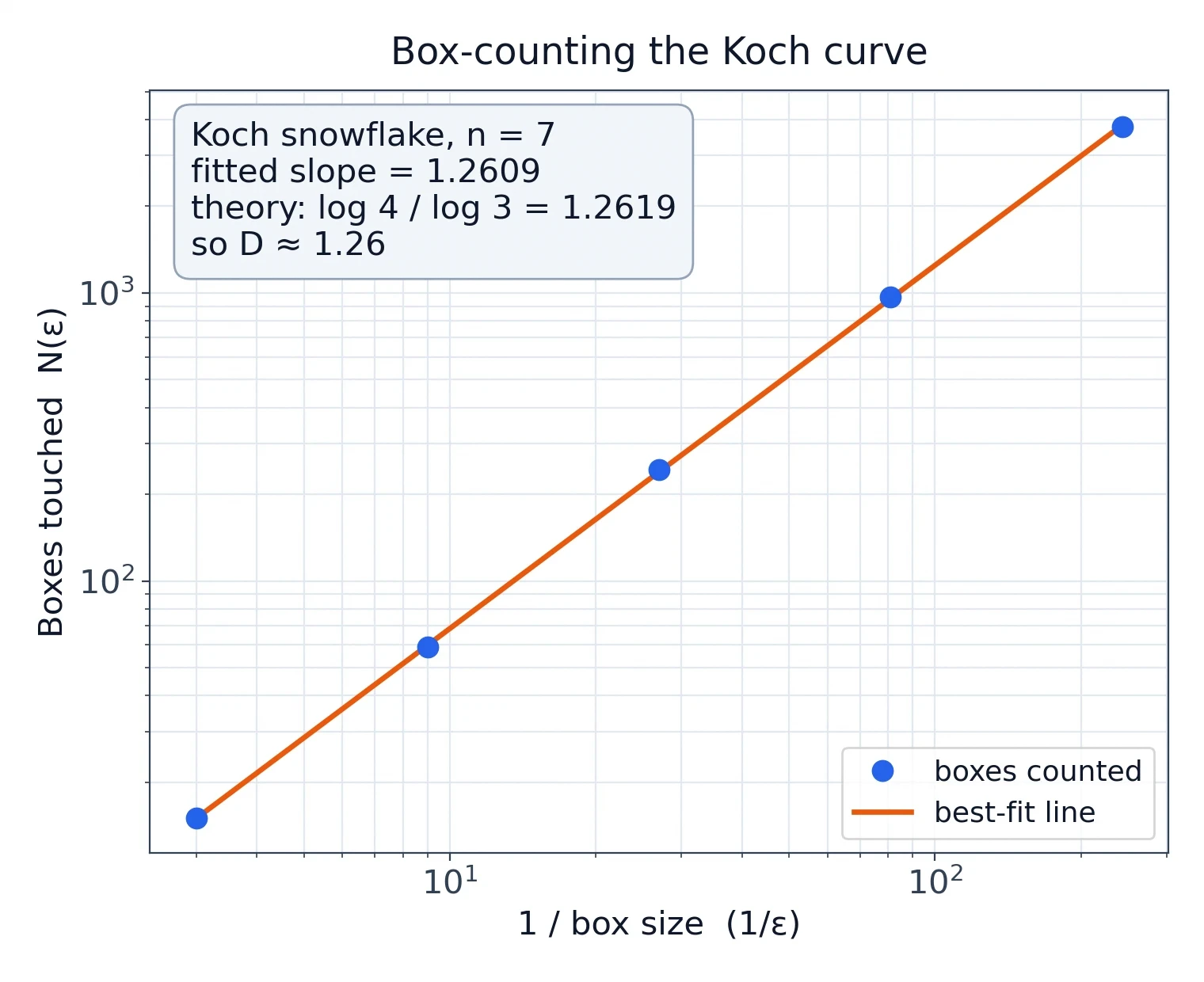
Apply the test to the Koch curve. Magnify a Koch curve by a factor of 3, and you need 4 copies of the original to build it — that is the construction itself, four segments of one-third size. So D equals log 4 divided by log 3, which is 1.2618595071, or about 1.2619. I recomputed this in Python, and the same computation gives the rest of the table:
| Fractal | Copies N | Scale factor S | Dimension log N / log S | Value |
|---|---|---|---|---|
| Koch curve | 4 | 3 | log 4 / log 3 | 1.2619 |
| Sierpinski triangle | 3 | 2 | log 3 / log 2 | 1.5850 |
| Sierpinski carpet | 8 | 3 | log 8 / log 3 | 1.8928 |
| Cantor set | 2 | 3 | log 2 / log 3 | 0.6309 |
| Menger sponge | 20 | 3 | log 20 / log 3 | 2.7268 |
Read the table as a ladder of roughness. Cantor's dust, at 0.6309, is sparser than a line. The Koch curve, at 1.2619, is rougher than a line but well short of a surface. The Sierpinski triangle, at 1.5850, is rougher still. The carpet, at 1.8928, is nearly a surface. The Menger sponge, at 2.7268, is nearly a solid. Each number says how thoroughly the shape fills the space it lives in, and each one is a precise, checkable quantity — not a metaphor, not a feeling, a number you can compute from the construction rule.
Hausdorff's 1918 definition — and what "dimension 2 boundary" means
The similarity dimension works for shapes built by exact copying, but nature does not copy exactly. Felix Hausdorff, in March 1918, gave a definition of dimension that works for any set at all. His paper, "Dimension und äusseres Mass", appeared in Mathematische Annalen, volume 79, pages 157 to 179. The idea is to measure a shape by covering it with tiny balls and watching how the total measure of the covering behaves as the balls shrink. The dimension is the threshold at which the measure flips from infinite to zero. For a smooth curve the threshold is 1. For the Koch curve it is 1.2619. For a surface it is 2.
Hausdorff's definition is what makes Mandelbrot's definition of a fractal work: a fractal is a set whose Hausdorff dimension strictly exceeds its topological dimension. The Koch curve is topologically a curve, dimension 1, but its Hausdorff dimension is 1.2619, so it counts as a fractal. A smooth circle has Hausdorff dimension 1, equal to its topological dimension, so it is not a fractal. The definition is crisp, and it draws the line exactly where intuition wants it drawn.
The most startling application of Hausdorff dimension in this whole subject concerns the boundary of the Mandelbrot set, which we will meet in Section 10. Mitsuhiro Shishikura proved that the boundary of the Mandelbrot set has Hausdorff dimension 2. The boundary is a curve — topologically one-dimensional — yet its Hausdorff dimension is 2, the dimension of a surface. It is so crinkled, so infinitely folded, that in the dimension sense it "fills" area, even though it has zero area itself. Read that again, slowly, because it is the single most counter-intuitive fact in this article: a curve can be so rough that its dimension is 2. Shishikura's proof was circulated as a preprint in 1991 and published in the Annals of Mathematics in 1998, volume 147, pages 225 to 267. The same paper shows that a typical Julia set for a point on the boundary also has Hausdorff dimension 2.
Box-counting: how you measure a real coastline
The copy-and-scale test needs exact copies, which nature does not provide. For real shapes — coastlines, clouds, lungs — the practical method is box-counting. Cover the shape with a grid of boxes of side length epsilon, and count how many boxes the shape touches. Make the boxes smaller and count again. If the count grows like epsilon to the power of negative D, then D is the box-counting dimension. In practice you plot the logarithm of the box count against the logarithm of the box size, and the slope of the straight line that fits the points is the dimension. That slope is what Figure 3 shows for the Koch curve.
This is the same idea as the logarithm test, turned into a measurement procedure. Instead of asking how many exact copies appear at a known scale, you ask how the count of boxes grows as the boxes shrink. The Cornell fractal dimension explainer walks through the same reasoning with clear diagrams, and it is a good companion to this section.
8. The Coastline Paradox, Solved — Almost
Richardson's rulers and the 20% border disagreement
Lewis Fry Richardson was a meteorologist and a pacifist who spent the 1920s and 1940s measuring things other people thought were already known. He measured the lengths of national borders and coastlines using rulers of different lengths, and he found a pattern that no one had written down before. As the ruler got shorter, the measured length got longer, and it got longer in a regular way: the length L measured with a ruler of length G follows L approximately equal to M times G to the power (1 minus D), where M is a constant and D is a number greater than or equal to 1. Double the precision of the ruler and the length grows by a predictable factor.
The border between Spain and Portugal made the point concretely. The two countries disagreed by roughly twenty percent about the length of their shared border, and the disagreement was not a matter of politics or error. Each side had measured with a different ruler length, and each side was right by its own ruler. Richardson's law says there is no single true length to disagree about. The border, like a coastline, has detail at every scale, and the measured length depends on the scale of the measurement.
Richardson published this work posthumously, in 1961, as "The problem of contiguity: An appendix to the statistics of deadly quarrels", in the General Systems Yearbook, volume 6, pages 139 to 187. He had been studying the statistics of war, and the border measurements were part of that larger project. The coastline paradox was, for him, a side observation. It became the founding observation of fractal geometry.
Mandelbrot's 1967 paper and D = 1.25 for Britain's west coast
Mandelbrot took Richardson's law and saw the dimension hiding inside it. In "How Long Is the Coast of Britain? Statistical Self-Similarity and Fractional Dimension", published in Science on 5 May 1967, volume 156, pages 636 to 638, he reinterpreted Richardson's exponent D as the coastline's fractional dimension. The ruler law becomes a statement about dimension: a coastline measured with a ruler of length G has length proportional to G to the power (1 minus D), and D is the dimension of the coast.
For the west coast of Great Britain, Mandelbrot gave D equal to 1.25. The number comes from Richardson's data, fitted to the ruler law. Mandelbrot's paper also reports other values from Richardson's measurements: the coastline of South Africa has D of about 1.02 — nearly smooth, almost a line — while lake shorelines typically come in around D equal to 1.28, rougher than Britain's west coast. A higher D means a rougher coast, one whose length grows faster as the ruler shrinks. A D near 1 means a coast that is nearly smooth at the scales measured.
The paper's title is a question, and the question is the point. "How long is the coast of Britain?" has no answer without a ruler length, and the honest answer is a dimension, not a length. The dimension tells you how the length changes with the ruler. That shift — from asking for a length to asking for a dimension — is the move that created fractal geometry.
What the paper did NOT claim
Here is the caution, and it matters. Mandelbrot's 1967 paper does not claim that any real coastline actually has a fractional dimension. It says Richardson's law is compatible with modelling coasts as random self-similar figures. Compatibility is not proof. A real coastline is a complicated product of geology, tides, erosion, and history, and a fractal model is a useful description of its roughness over a range of scales, not a claim about what the coastline fundamentally is.
9. Fractals in Nature: Real, Approximate, and Finite
Trees, rivers, and lightning: branching that fills space
Look at a tree in winter, when the leaves are gone. A trunk splits into limbs. Each limb splits into branches. Each branch splits into twigs. Each level resembles the last, only smaller. The pattern is not exact — no two branches are identical — but the structure repeats: a thick channel splitting into thinner channels, again and again, until the twigs are thin as wire. The same branching shows up in roots underground, in river networks where small streams join into larger channels, in lightning bolts forking across the sky, and in the cracks that spread through drying mud or breaking ice.
Why does nature keep using this pattern? Because branching is an efficient way to fill space and to move things around. A tree needs to deliver water from its roots to every leaf and to collect sunlight across a wide canopy, and a branching network does both with a minimum of material. A river network needs to drain a whole landscape into a single outlet, and branching does it. A lung needs to bring air into contact with blood across a huge surface, and branching does it. The fractal pattern is not a decoration. It is a solution to a transport problem, and evolution and physics keep rediscovering it.
One caution belongs here, and I want to state it plainly. No verified "tree fractal dimension" number exists in the research behind this article. Published estimates vary by species and by measurement method, and none of them was checked against a primary source for this article. So I will not quote one. The branching pattern is real and visible. A single number for "the dimension of a tree" would be false precision, and this article does not do false precision.
Ferns and snowflakes: the pattern you can hold in your hand
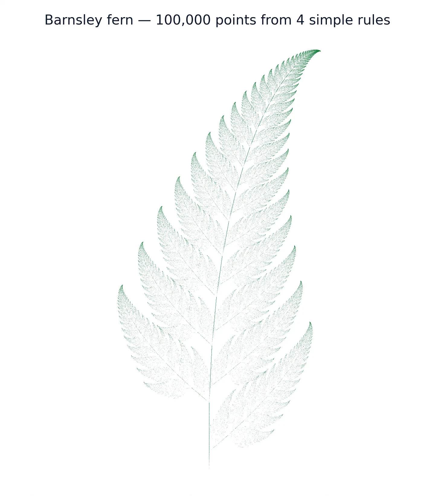
A fern frond is the clearest plant example of self-similarity you can hold in your hand. Each leaflet along the frond resembles a small copy of the whole frond, with its own smaller leaflets arranged the same way. Hold a frond up, look at a leaflet, and you see the frond again, smaller. The resemblance is approximate — real ferns are messier than the mathematics — but it is unmistakable, and it is why the fern became the emblem of fractal geometry. The Barnsley fern of Section 12 reproduces this pattern with four simple rules, and the match is good enough that the computer-drawn fern is hard to tell from a photograph at a glance.
Snowflakes are the other classic. A snowflake grows by diffusion: water vapour freezes onto a tiny ice crystal, and the crystal grows arms in six directions. Each arm grows side-branches, and each side-branch echoes the arm. The result is a six-fold pattern with detail at several scales, and no two snowflakes are alike because the growth conditions — temperature, humidity, the exact path through the cloud — differ every time. A snowflake is a finite fractal: growth stops when the flake falls, and there is no infinite regress. The pattern repeats over a few scales and then the physics runs out. That is the honest story, and it is beautiful enough without exaggeration.
The same warning applies to the golden ratio here as it does everywhere in this cluster. A nautilus shell is often presented as a golden-ratio or fractal example, and it is not. The shell is a logarithmic spiral, and its growth does not follow the golden ratio. Our article on the golden ratio explains the nautilus myth in full. Do not let a pretty spiral do the work of evidence.
Your lungs: 480 million alveoli and the tennis-court correction
Your lungs are the most dramatic fractal in your own body, and the numbers are worth getting right, because the most famous version of them is wrong. Adult human lungs contain about 480 million alveoli — the tiny air sacs where oxygen passes into the blood — on average, with a range of roughly 274 to 790 million between individuals, scaling with lung size. Those figures come from Ochs and colleagues, published in 2004 in the American Journal of Respiratory and Critical Care Medicine, volume 169, pages 120 to 124, and summarised in Kenhub's alveoli reference. The total alveolar surface area is about 70 to 75 square metres in adults.
Now the famous claim. You will often read that the surface area of your lungs, spread flat, would cover a tennis court. It is a vivid image, and it is wrong by a factor of about four. A doubles tennis court is 23.77 metres by 10.97 metres, which is about 260.8 square metres. Seventy square metres is about 0.27 times that — roughly one quarter of a tennis court, not a whole one. A better comparison is a badminton court, which is about 81.7 square metres: your lungs' surface is about 0.86 times a badminton court, nearly the whole thing. The tennis-court version of the claim has been repeated so often that it feels true, and it is a good reminder that a vivid comparison is not the same as a checked number. I checked this one myself with a calculator, and the arithmetic is not close: 70 divided by 260.8 is 0.27, and no rounding will turn that into 1.
A quick sanity check supports the published area. An alveolus is roughly a sphere about 0.2 millimetres across. Take 480 million of them, multiply by the surface area of a sphere of radius 0.1 millimetres, and you get about 60 square metres — the same order of magnitude as the published 70 to 75. The numbers hang together. The lungs achieve that enormous surface inside a chest cavity because the airways branch again and again, each generation thinner and more numerous, until the air reaches the alveoli. The branching is fractal in structure over the range from the trachea down to the smallest airways, and it stops where the anatomy stops: at cells, not at infinity.
Blood vessels, Romanesco broccoli, clouds, and mountains
Blood vessels branch the way trees do: a large vessel splits into smaller ones, again and again, until the finest capillaries feed single cells. A Romanesco broccoli shows the same idea on a dinner plate — each floret is a small cone made of smaller cones, spiralling in the same pattern at every scale. Clouds and mountains are the classic cases for computer graphics, where fractal algorithms generate their roughness: a mountain range built this way looks real from any distance, because the roughness repeats at every scale. None of these is an exact fractal. A real blood vessel has a smallest size, a real cloud has a smallest droplet, and the repetition always stops. What they share is roughness over a range of scales — and the fractal dimension gives that roughness a number.
The honest limit: nature stops repeating
All of this needs the frame it opened with. Natural fractals are approximate, finite, and scale-limited. No real coastline, tree, or lung repeats forever. A tree's branching stops at twigs and leaves. A coastline's detail stops at grains of sand and then at atoms. A lung's branching stops at cells. Fractal geometry is a model of roughness over a range of scales, not a claim that nature runs an infinite algorithm.
That limit is not a disappointment. It is what makes the model useful. Saying "this coastline behaves like a fractal between one kilometre and one hundred kilometres, with dimension about 1.25" is a precise, testable, useful statement. Saying "nature is fractal" is a slogan. Science runs on the first kind of sentence, and this article will keep using it.
10. The Mandelbrot Set: One Tiny Rule, Infinite Beauty
Complex numbers in one paragraph (link to Imaginary Numbers #16)
Everything in this section runs on complex numbers, and here is all you need. A complex number has two parts: a real part and an imaginary part, written as a plus b times i, where i is the square root of negative one. You can picture it as a point on a flat plane, with the real part as the horizontal coordinate and the imaginary part as the vertical coordinate. Adding and multiplying complex numbers is just arithmetic on the two parts, following the rule that i squared equals negative one. That is the whole toolkit. If solving equations with unknowns feels rusty, our article on how algebra works builds the skill from the ground up. If you want the full story — why imaginary numbers are not imaginary at all, and how they earned their place in mathematics — our article on imaginary numbers tells it properly.
The rule: z → z² + c, starting from zero
The Mandelbrot set is built from one rule. Pick a complex number c. Start with z equal to zero. Then repeat: replace z with z squared plus c. That is it. One squaring, one addition, repeated forever. The question is what happens to z as you keep going. For some choices of c, the values of z stay small forever, bouncing around near the origin. For others, the values run away to infinity, growing without bound. The Mandelbrot set is the set of all c for which the values stay bounded forever.
The starting point matters, and it is worth pausing on. We always start from z equal to zero. Zero is the seed, the same for every c. That is why the Mandelbrot set is a picture of the parameter c, not of the starting point: we fix the start and vary the rule, by varying c. The contrast with Julia sets, where we fix c and vary the start, is the subject of Section 11. The number zero, the starting point of the whole picture, is also the subject of our article on the history of zero, which is a good companion piece for anyone who finds it strange that so much can grow from nothing.
The escape test: if |z| passes 2, it never comes back
You might think that deciding whether an orbit stays bounded forever would take forever to check. It does not, because of a clean escape test. If at any step the size of z — its distance from the origin, written as |z| — passes 2, then the orbit escapes to infinity for certain. It will never come back. The squaring takes over from that point, and each step roughly squares the size, so the values explode.
That test is what makes the Mandelbrot set drawable. A computer picks a point c, iterates the rule, and watches |z|. If |z| passes 2, the point is outside the set, and the number of steps it took to escape decides the colour. If |z| stays at or below 2 for, say, a few hundred steps, the point is treated as inside the set and coloured black. The whole set lies inside the disk where |c| is less than or equal to 2, and its intersection with the real axis is exactly the interval from negative 2 to 0.25. Those bounds are proven facts, not guesses, and they frame the picture: the set is a compact blob, a little over two units wide, sitting on the real axis between negative 2 and 0.25.
Worked orbits: c = 1 escapes, c = −1 cycles, c = 0.25 creeps
The best way to feel the rule is to run it by hand for a few values of c. I recomputed all of these orbits in Python, and you can check each step with a pocket calculator.
Take c equal to 1. Start at 0. Then 0 squared plus 1 is 1. Then 1 squared plus 1 is 2. Then 2 squared plus 1 is 5. Then 5 squared plus 1 is 26. The values are already past 2 at the third step, and they explode from there. The point c equal to 1 is not in the Mandelbrot set.
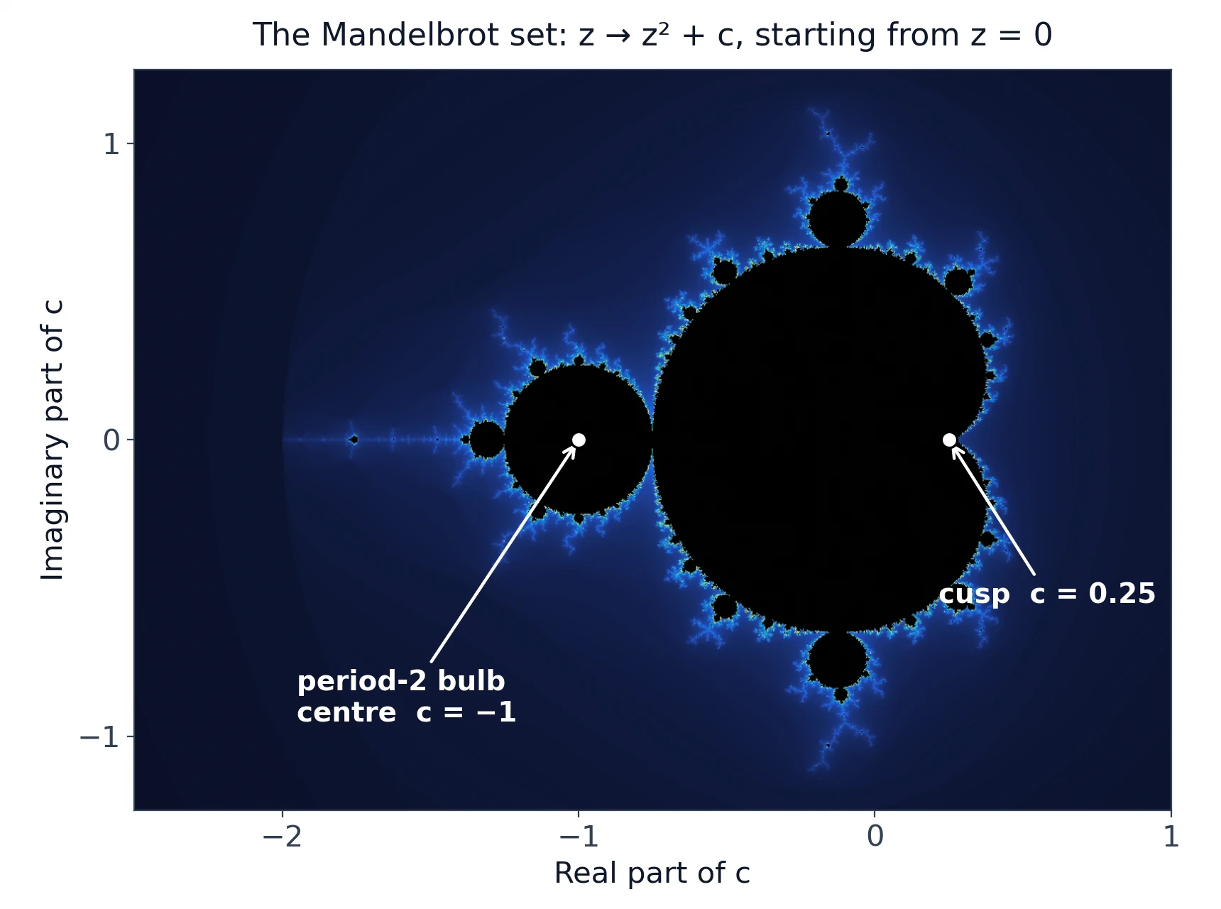
Take c equal to negative 1. Start at 0. Then 0 squared minus 1 is negative 1. Then negative 1 squared minus 1 is 0. Then 0 squared minus 1 is negative 1 again. The orbit cycles: 0, negative 1, 0, negative 1, forever. It never escapes, so c equal to negative 1 is in the set. It is, in fact, the centre of the period-2 bulb, the round region to the left of the main cardioid, and we will meet it again below.
Take c equal to 0.25, the cusp of the main cardioid. The orbit goes 0, 0.25, 0.3125, 0.3477, 0.3709, and keeps creeping slowly upward toward 0.5, the fixed point. It never escapes. The creep is slow — the orbit approaches its limit like a tired walker — and that slowness is characteristic of points near the cusp. They are in the set, but only just, and a computer needs many iterations to be sure.
One more orbit is worth a careful look, because it corrects a common mistake — one this article nearly made itself. Take c equal to negative 0.75 plus 0.1i. Over twenty iterations the size of z stays below 1 throughout — the values run 0.7566, 0.2037, 0.7235, 0.2649, and so on, never settling quickly, never escaping — and twenty iterations look like enough to call the point inside the set. They are not. Keep going and the orbit escapes at iteration 33, when z reaches about negative 0.75 plus 2.60i, a size of about 2.70, past the escape threshold of 2. The point sits in a filament gap outside the set, not inside it. Twenty iterations cannot establish membership: a point is only treated as inside after hundreds of iterations with no escape. The distance-from-negative-1 arithmetic still holds — the point sits about 0.269 from negative 1, just past the period-2 bulb's radius of 0.25 — but being outside the bulb does not mean being inside the set, and that is exactly the distinction sloppy writing conflates.
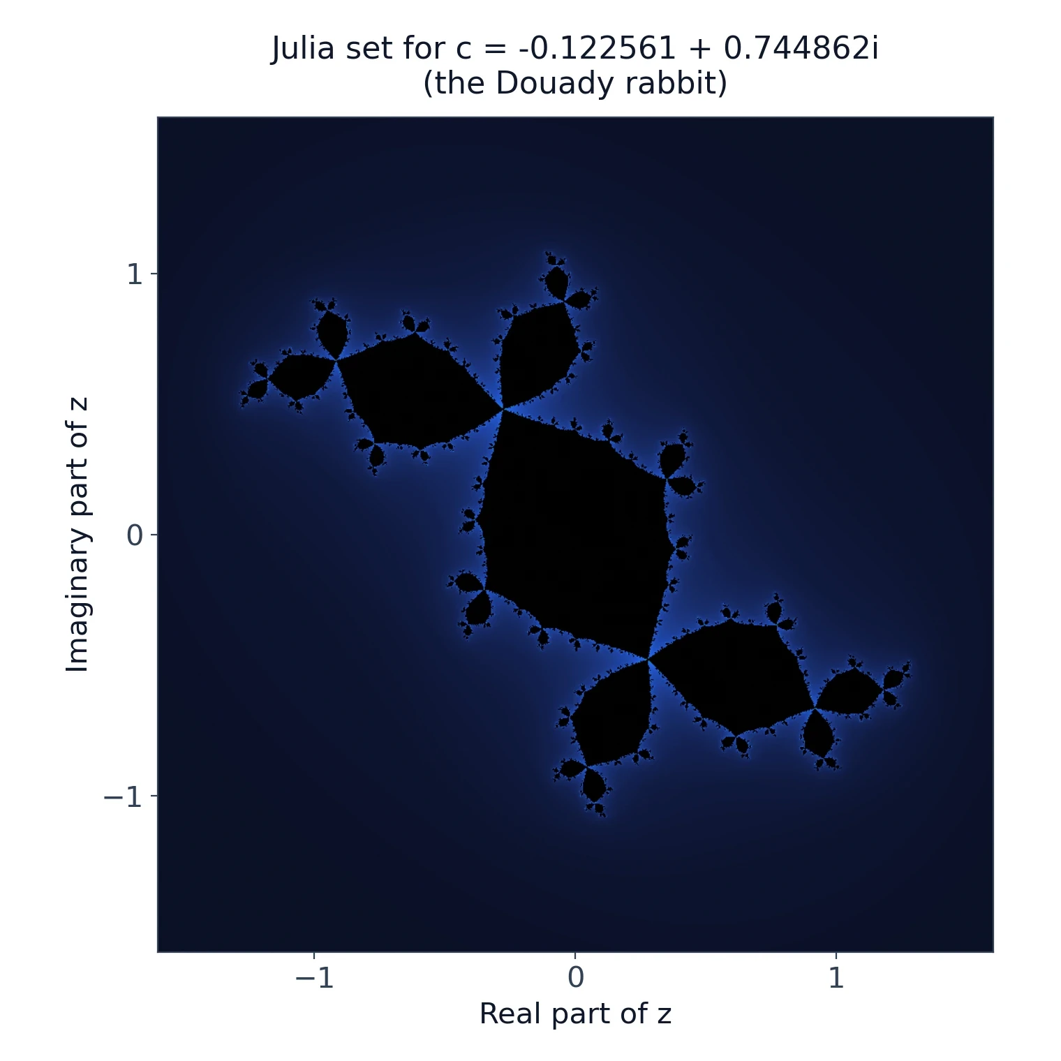
A genuinely bounded example with the same wandering flavour is the centre of the period-3 bulb, c approximately equal to negative 0.122561 plus 0.744862i. Its orbit closes exactly after three steps: 0, then c, then c squared plus c — about negative 0.662359 plus 0.562280i — and then back to 0, repeating forever. It never escapes, so this point is in the set. We will meet it again in Section 11, where its Julia set has a name: the Douady rabbit.
Reading the picture: cardioid, period-2 bulb, mini-Mandelbrots
The picture itself, Figure 5, is the most famous image in mathematics, and it repays a guided reading. The big heart-shaped region in the middle is the main cardioid. Points c inside it give an orbit that is attracted to a fixed point — a period-1 cycle, the orbit settling to a single value. The cusp of the cardioid is at c equal to 0.25, the creeping point we just computed. The cardioid can be described exactly: c equals lambda over 2 minus lambda squared over 4, for lambda with size less than 1.
Attached to the left of the cardioid is a round bulb, the period-2 bulb. Its centre is c equal to negative 1, its radius is 1/4, and on the real axis it covers the interval from negative 5/4 to negative 3/4. Inside it, the orbit is attracted to a period-2 cycle, bouncing between two values the way the orbit of negative 1 bounces between 0 and negative 1. Smaller bulbs sprout from the cardioid and from the period-2 bulb, each one corresponding to a cycle of a different period: period-3 bulbs attach to the top and bottom of the cardioid at c approximately equal to negative 0.125 plus 0.6495i and its mirror image below the real axis, with their centres near c approximately equal to negative 0.123 plus 0.745i and its mirror image. Every bulb is a region where the orbit settles into a cycle of a fixed period, and the bulbs fit together like bubbles on the surface of the set.
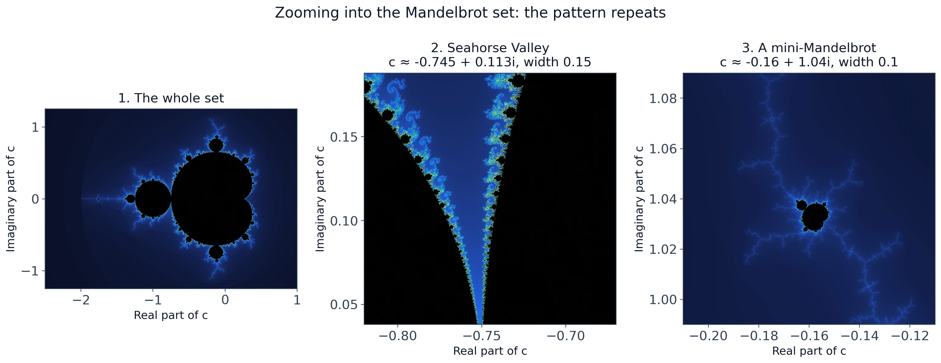
Zoom into the filaments — the thin, branching threads that sprout from the bulbs — and you find mini-Mandelbrots: small copies of the whole set, complete with their own cardioids and bulbs, sitting in the tendrils. There are infinitely many of them, at every scale, and zooming in never exhausts them. That is self-similarity at its most dramatic: the set contains copies of itself, and those copies contain copies of themselves.
The first time I watched a Mandelbrot zoom on a screen, the image falling inward through scale after scale, each level revealing a new miniature of the whole, I felt the same vertigo I had felt with the coastline and the string. A shape made by one rule, repeating forever, with no bottom to it. The computer was drawing it in real time, and the picture kept giving. That is the moment, I think, when most people understand what a fractal is — not from a definition, but from watching the zoom refuse to end.
The area of the Mandelbrot set is estimated at about 1.51 — a small fraction of the disk of radius 2 that contains the whole set, whose area is 4 times pi, about 12.57. That number is a numerical estimate from pixel-counting computations, current as of October 2012, and the exact area is unknown. It must be presented as an estimate, not as an exact value. The boundary, meanwhile, has Hausdorff dimension 2, as Shishikura proved — the fact we met in Section 7. A curve with the dimension of a surface, bounding a region of area about 1.51, generated by one line of arithmetic. There is nothing else in mathematics quite like it.
"Clouds are not spheres, mountains are not cones, coastlines are not circles, and bark is not smooth, nor does lightning travel in a straight line." — Benoît Mandelbrot, The Fractal Geometry of Nature (1982), p. 1.
11. Julia Sets: One Rule, Infinitely Many Pictures
Fix c, vary the starting point: the other half of the story
The Mandelbrot set fixes the starting point at zero and varies c. A Julia set does the opposite: it fixes c and varies the starting point. For a chosen value of c, the Julia set is the boundary between the starting points z whose orbits under z going to z squared plus c stay bounded, and the starting points whose orbits escape to infinity. Same rule, different question. The Mandelbrot set asks, for each rule, does the orbit from zero stay bounded? A Julia set asks, for one rule, which starting points stay bounded?
That swap produces infinitely many different pictures. Every value of c gives a different Julia set, and the variety is astonishing: some are connected blobs, some are delicate dendrites like bare winter trees, some are spirals that look like galaxies, some are scattered dust. The Mandelbrot set is one picture. The Julia sets are an infinite gallery, all generated by the same rule.
Connected or dust: the Mandelbrot set as an index
Here is the deep connection between the two. If c lies inside the Mandelbrot set, its Julia set is connected — one piece, unbroken. If c lies outside the Mandelbrot set, its Julia set is totally disconnected, a scattered dust of points, a Cantor-like scatter that mathematicians call Fatou dust. The Mandelbrot set is therefore an index, a map, of all the Julia sets: it tells you, for each c, whether the corresponding Julia set holds together or falls apart.
That is a remarkable fact, and it is why the two sets are always discussed together. The Mandelbrot set is not just a pretty picture. It is the catalogue of a whole infinite family of shapes, and its boundary is the dividing line between connection and dust. The points on the boundary itself give the most interesting Julia sets of all — the dendrites and spirals, the shapes that are connected but only just, hanging together by threads.
Julia and Fatou, 1918 — the pictures nobody could see
Gaston Julia was a French mathematician who, in 1918, published a 199-page memoir, "Mémoire sur l'itération des fonctions rationnelles", in the Journal de Mathématiques Pures et Appliquées, 8th series, volume 1, pages 47 to 245. He was twenty-five, and he had been wounded in the First World War, wearing a leather mask over part of his face for the rest of his life. His memoir worked out the theory of iterating rational functions — the mathematics behind Julia sets — in full generality, without ever seeing a picture of one. He won the Grand Prix of the French Academy of Sciences for it in 1918.
The Douady rabbit and other famous Julia sets
The most famous Julia sets have names. The Douady rabbit is the Julia set for c approximately equal to negative 0.122561 plus 0.744862i — the centre of the period-3 bulb, the same point whose exact three-step orbit we computed in Section 10. Its shape has ear-like lobes that suggest a rabbit's head, and it is connected, as the theory says it must be, because c lies inside the Mandelbrot set. Other famous examples include the dendrite for c equal to i, on the boundary of the Mandelbrot set, whose Julia set is a branching tree with no interior at all — connected, but only just, hanging together by threads.
A word of caution belongs here. Every c value named in this section was verified numerically before it was written down: the rabbit's c was checked to ten thousand iterations with no escape, and its orbit closes exactly after three steps; the dendrite's c equal to i was checked the same way. A Julia set should be verified by rendering it, not by trusting a list. Figure 7 shows the verified one, the rabbit, with its c value printed from the render code.
12. How Fractals Are Drawn: Iteration, IFS, and the Chaos Game
Iteration: the same step, forever
Every fractal in this article is built by iteration: take a step, apply the same rule to the result, and repeat. The Koch snowflake iterates a geometric rule on edges. The Sierpinski triangle iterates a removal rule on triangles. The Mandelbrot set iterates a formula on numbers. The rule never changes. What changes is the input, and the input is always the previous output.
Iteration is the engine of the whole subject, and it is worth noticing how little machinery it needs. A rule, a starting point, and repetition. The complexity does not come from a complicated rule. It comes from repetition itself, from the way a small change in one round is amplified by the next. That is also why fractals connect so naturally to chaos theory, which is the subject of Section 13 and of our article on chaos theory.
Iterated function systems and the Barnsley fern (4 maps, 24 numbers)
An iterated function system, or IFS, is a set of contraction mappings — rules that shrink and move shapes — applied repeatedly, with the fractal emerging as the attractor that the process converges to. The idea was developed by Michael Barnsley and Stephen Demko in a 1985 paper, and Barnsley's book Fractals Everywhere, published in 1988, made it the standard method for generating fractals from a handful of rules.
The showcase is the Barnsley fern. Four affine transformations — each one a combination of scaling, rotation, and shifting — applied with probabilities 0.01, 0.85, 0.07, and 0.07, generate a fern that looks startlingly like a real one. The four maps play four roles: the stem, the main frond, the left leaflets, and the right leaflets. The whole fern is encoded in 24 numbers — four maps, six coefficients each — plus the four probabilities, making 28 parameters in total. Saying "24 numbers" without the probabilities, or "28 parameters" without explaining the split, would both be misleading, so here is the honest version: 24 coefficients plus 4 probabilities. A few dozen numbers describe a fern that would take roughly a megabyte to store as a bitmap image. That compression is not a party trick. It is the reason fractal image compression was taken seriously, and Section 14 will come back to it.
The Barnsley fern's fractal dimension is reported in the literature as about 1.74. That value was not independently recomputed in the research for this article, so the honest statement is that the dimension is about 1.7. It sits between a line and a surface, as a fern should: more than a curve, less than a solid sheet.
The chaos game: randomness that draws exact order
The chaos game, which we met in Section 6 as a way of drawing the Sierpinski triangle, deserves a closer look, because it is the clearest demonstration in the subject that randomness and order are not opposites. The procedure is simple: pick a random vertex, jump halfway toward it, plot a point, and repeat. The randomness is real — a die roll, a random number generator, a coin — and the result is exact: the points converge onto the Sierpinski triangle, the same shape the removal rule builds. The mathematics of that randomness — what 'random' means, and how to measure it — is the subject of our article on probability.
Why computers were the missing ingredient (1979–1980)
All of this explains why fractals waited so long to be seen. The mathematics of iteration existed by 1918. The pictures did not, because no human can iterate a rule ten thousand times and plot the results by hand. Mandelbrot's visualisation of the Mandelbrot set in 1979 and 1980, on IBM computers, was the moment the field became visible — literally. The computer was not a convenience. It was the missing ingredient, the tool that turned a theory about iteration into a picture you could look at, zoom into, and explore.
Figure 8 shows the chaos game in action: a Sierpinski triangle drawn by random half-way jumps, about fifty thousand points plotted by code, beside the same triangle built by the removal construction. Two processes, one deterministic and one random, converging on one shape. That convergence is the thesis of this section in a single image.
13. Fractals Meet Chaos
Lorenz 1963 and the butterfly that never repeats
In March 1963, Edward Lorenz published "Deterministic Nonperiodic Flow" in the Journal of the Atmospheric Sciences, volume 20, pages 130 to 141. He had been running a simplified model of atmospheric convection on a computer — three equations, three variables — and he found something that should not have been possible. The model was deterministic: the same starting point always gives the same result. But the motion never repeated itself. It wandered forever around a strange, butterfly-shaped region of the state space, never settling into a cycle, never repeating a path.
That shape, the Lorenz attractor, is a fractal. Its dimension is about 2.06 — just above 2, a surface with extra roughness, a shape that is almost a surface but never quite fills one. The trajectory winds around two lobes like a butterfly's wings, switching lobes unpredictably, never crossing itself, never repeating. It is deterministic and unpredictable at the same time, and the reason is sensitivity to initial conditions: two starting points that differ by a hair follow paths that diverge exponentially, until they have nothing in common.
Strange attractors have fractal shape
Lorenz's discovery was the birth of chaos theory, and the fractal shape of the attractor is not a coincidence. A chaotic system needs somewhere for its trajectories to go, and that somewhere has to be bounded — the motion cannot run away to infinity — but it also has to be roomy enough that trajectories never repeat. A smooth shape cannot do both. A fractal can. Its infinite detail gives the trajectories endless room to wander without ever retracing a step, inside a bounded region.
The same mathematics, two different questions
Fractals and chaos are often confused, and the confusion is understandable, because they share the same engine: iteration. But they ask different questions. Fractal geometry asks: what shape does this rule build, if I repeat it forever? Chaos theory asks: what does this system's behaviour look like over time, and how sensitive is it to where it starts? The Mandelbrot set is a fractal question. The Lorenz attractor is a chaos question. The two meet because the answer to the chaos question so often turns out to be a fractal shape.
Our article on chaos theory tells the Lorenz story in full, including the weather model, the butterfly effect, and the question of whether long-term weather prediction is possible at all. This article's contribution is the geometric half of the story: the shape that chaos lives on is a fractal, and the dimension of that shape — about 2.06 for Lorenz — is the number that says how thoroughly chaos fills its space. Read the two articles together and the connection is complete.
14. What Fractals Are Good For
Antennas that fit in your phone (Cohen, 1988)
In 1988, Nathan Cohen, a radio astronomer in Boston, built the first fractal antenna because his flat's lease forbade an outdoor antenna. He cut a Koch-curve pattern from foil on a sheet of A4 paper, and it worked — better, in some ways, than a conventional antenna of the same size. The reason is self-similarity: a fractal antenna resonates at several frequencies at once, because its structure repeats at several scales, and each scale picks up a different band. A conventional antenna is tuned to one frequency. A fractal antenna is tuned to several, and it is smaller, because the fractal packs more length into a smaller area — the same property that gives the Koch snowflake its infinite perimeter.
Cohen founded Fractal Antenna Systems in 1995, and his work was patented in the United States as patent 6,452,553, filed in 1995 and granted on 17 September 2002. Fractal antennas now appear in mobile phones and other compact devices, where space is short and several frequency bands must be served by one small element. The Koch curve, a mathematical curiosity from 1904, became an engineering component because its geometry solves a real packaging problem.
Squeezing pictures: fractal image compression (Barnsley, 1988)
The same year, 1988, Barnsley and Alan Sloan described fractal image compression in the January issue of BYTE magazine, in an article called "A better way to compress images". The idea was the Barnsley fern in reverse: instead of generating a picture from a few numbers, find the few numbers that generate a given picture. Store the rules, not the pixels, and the image compresses dramatically. The method was patented in the United States as patents 4,941,193 in 1990 and 5,065,447 in 1991, and it was used in Microsoft Encarta and in CD-ROM encyclopaedias in the 1990s.
Mountains and clouds on screen: fractal graphics
Fractal terrain is the application most people have seen without knowing it. Mountains and clouds in films and video games are often generated by fractal methods: midpoint displacement, in which a line is repeatedly subdivided and its midpoints pushed up or down by random amounts, produces ridgelines that look like real mountains at every scale. Clouds are generated the same way, with fractal noise giving the ragged edges that smooth shapes cannot produce.
Markets that do not follow the bell curve (Mandelbrot 1963, fat tails)
In 1963, Mandelbrot published "The Variation of Certain Speculative Prices" in the Journal of Business, volume 36, pages 394 to 419. He had been studying cotton prices, and he found that they do not follow the bell curve. Extreme moves — huge jumps in price — happen far more often than the normal distribution predicts. The distribution has "fat tails": rare events are not rare enough. He also found that price charts look statistically similar at different time scales: a chart of daily prices resembles a chart of monthly prices, the same statistical roughness repeated across scales. That is statistical self-similarity, the same idea as the coastline, applied to money.
This matters because most financial models assume the bell curve. If prices have fat tails, the models underestimate risk, and they underestimate it exactly where it hurts: in the rare, huge moves. Our article on the normal distribution explains the bell curve and its assumptions in full, and the contrast is the point: the bell curve is a beautiful model, and markets are rougher than it. Mandelbrot collected this work in Fractals and Scaling in Finance in 1997, and wrote a popular account with Richard Hudson, The (Mis)Behavior of Markets, in 2004.
One caution, stated plainly: fractal models describe the statistics of wildness. They do not forecast prices. Anyone who tells you that fractals predict the market is selling something. What they do is tell you honestly how wild the market is, and how wrong the smooth models are about that wildness.
Medicine: reading roughness in tumours, retinas, and heartbeats
Fractal dimension has become a diagnostic signal in medicine. The roughness of a tumour's boundary, the branching of blood vessels in the retina, the variability of a heartbeat over time, the structure of bone: each of these can be summarised by a fractal dimension, and changes in that number can signal disease. A tumour with a rougher boundary, a retina whose vessels have lost their normal branching pattern, a heartbeat whose variability has become too regular or too wild — each is a case where the roughness number carries information that a doctor can use.
15. What Fractals Are Not
Myth 1: everything in nature is a fractal
Most people assume that once you learn what a fractal is, you start seeing fractals everywhere — in every tree, every cloud, every coastline, every snowflake. What the evidence actually shows is narrower and more interesting. Some natural shapes behave like fractals over some range of scales, and some do not. A coastline does, between kilometres and hundreds of kilometres. A tree's branching does, over a few generations. A cloud's edge does, over the scales a photograph can resolve. But a pebble is not a fractal. A calm lake is not a fractal. A single leaf, looked at closely, is mostly smooth.
The claim "everything in nature is a fractal" is wrong in the same way that "everything in nature is a circle" would be wrong. It takes a useful idea and stretches it until it means nothing. The honest claim is always specific: this shape, over this range of scales, with this dimension, measured this way. That is a smaller claim, and it is a true one, and it is worth more than the slogan.
Myth 2: the Mandelbrot set proves the universe is a computer
The Mandelbrot set is so beautiful, and so clearly generated by a rule, that it tempts people into a grand conclusion: if a simple rule can generate infinite beauty, then perhaps the universe itself is a computer program, running a simple rule. That is a philosophical claim, not a mathematical one, and the Mandelbrot set does not support it. It shows that a simple rule can generate infinite complexity. It does not show that the universe is generated by a simple rule. Those are different statements, and the second does not follow from the first.
Myth 3: fractal dimension is the same as "complexity"
Fractal dimension is often described as a measure of complexity, and that description is misleading. Dimension measures roughness, or space-filling, over a range of scales. A shape can be rough and simple — the Koch curve is built from one rule — or smooth and complex, like a machine with a thousand parts and a dimension of exactly 3. Complexity and roughness are different properties, and a single number cannot measure both.
The confusion matters because it leads people to compare dimensions across shapes that were measured differently and conclude that one is "more complex" than another. A coastline with dimension 1.25 and a lung with dimension about 1.7 are not in a complexity contest. They are rough in different ways, at different scales, for different reasons. The number is useful when you compare like with like — two coastlines, two tumours, two heartbeats — and misleading when you treat it as a universal score.
The open question: is the Mandelbrot set locally connected?
The biggest open question in the subject is whether the Mandelbrot set is locally connected, usually abbreviated MLC. Local connectedness means that every point of the set has arbitrarily small neighbourhoods, within the set, that are connected. It is a technical property, but it has a plain meaning: does the set hang together at every scale, with no point where the local structure falls apart into dust?
Nobody knows. It is a conjecture, not a theorem. It has resisted proof for decades, and it is connected to deep questions about the dynamics of quadratic polynomials. If it were proved, it would complete the picture of the Mandelbrot set in an important way. Until then, the honest statement is that it is conjectured, and the conjecture is one of the most famous open problems in the field. That is not a failure. It is a sign that a shape generated by one line of arithmetic still has secrets, more than forty-five years after it was first drawn.
16. The Pattern That Never Ends
What to remember: one rule, repeated, makes infinity
If you remember one thing from this article, let it be this: a simple rule, repeated forever, can make something infinitely rich. The Koch snowflake comes from cutting a middle third and adding a tent. The Sierpinski triangle comes from removing a middle quarter. The Mandelbrot set comes from squaring and adding. None of these rules is complicated. All of them, repeated without end, produce shapes with infinite detail, fractional dimension, and properties that seem impossible until you do the arithmetic.
The other thing is the number. Fractal dimension turns roughness into a quantity you can measure, compare, and use — in a coastline, a tumour, a heartbeat, a price chart. That is the real gift of the subject. It gave roughness a number, and once roughness had a number, it could be studied like anything else.
Where to go next: paradoxes, graph theory, and the rest of the cluster
The next article in this cluster takes up mathematical paradoxes — the statements and shapes that break intuition, including the ones this article only nodded at, like a curve of infinite length enclosing a finite area. After that comes graph theory, the mathematics of networks, which turns out to share a habit of mind with fractals: both reward looking for the simple rule underneath the complicated picture.
Both are coming in this Mathematics cluster, in the same style as this article: worked numbers, verified sources, and pictures you can check. If you want to go deeper right now, the Sources below are the place to start — Mandelbrot's 1967 coastline paper is short, readable, and still the best first step into the subject.
Try it yourself: three rules you can run on paper
You do not need a computer to meet a fractal. Take a sheet of paper and try these three.
First, the Koch rule. Draw an equilateral triangle. Divide each side into thirds, erase the middle third, and draw a small outward tent on each gap. Do it again on every new edge. Two iterations are enough to see the snowflake emerging, and your wrist will tell you why the third iteration is hard.
Second, the chaos game. Draw a large triangle on graph paper and label its corners A, B, and C. Pick any starting point inside. Roll a die: 1 or 2 means A, 3 or 4 means B, 5 or 6 means C. Move halfway from your point toward the chosen corner and mark a dot. Repeat, fifty times or a hundred. The Sierpinski triangle will appear out of your random jumps, and it will feel like a trick even though you did it yourself.
Third, the Mandelbrot rule. Pick c equal to negative 1 and iterate z going to z squared plus c from zero, on a calculator: 0, negative 1, 0, negative 1. Then try c equal to 1: 0, 1, 2, 5, 26, gone. Then try c equal to 0.25 and watch it creep toward 0.5. Three values of c, three fates, one rule. If you want to go further, a few lines of code will draw the whole set, and the picture that emerges is the one in Figure 5. It is yours to explore, one zoom at a time, and it does not end.
Frequently Asked Questions
What is a fractal?
A fractal is a shape with self-similarity, detail at every scale, and a dimension that is not a whole number, usually generated by a simple rule repeated forever. A small piece of a fractal looks like the whole shape, or nearly like it, and zooming in keeps revealing new structure. The Koch snowflake, the Sierpinski triangle, and the Mandelbrot set are the classic examples, and coastlines, ferns, and lungs are natural shapes that behave like fractals over a range of scales.
What is the Mandelbrot set?
The Mandelbrot set is the set of complex numbers c for which the iteration z going to z squared plus c, starting from z equal to zero, stays bounded forever. It is drawn by testing each point c: if the orbit escapes past size 2, the point is outside the set; if it stays bounded, the point is inside. The picture shows a large cardioid, round bulbs for cycles of different periods, and infinitely many miniature copies of the whole set in its filaments.
What is self-similarity?
Self-similarity means that a part of a shape resembles the whole shape. Exact self-similarity, in mathematical fractals like the Koch curve, means a magnified part is an identical copy. Approximate self-similarity, in ferns and trees, means parts resemble the whole with variation. Statistical self-similarity, in coastlines and clouds, means the statistics of the roughness repeat across scales even though no two stretches match.
Do fractals appear in nature?
Yes, but approximately and over a limited range of scales. Coastlines, trees, ferns, snowflakes, lungs, and river networks all show fractal-like branching or roughness over some range. No natural fractal repeats forever: a tree's branching stops at twigs, a coastline's detail stops at grains of sand, and a lung's branching stops at cells. The honest statement is always "fractal over this range of scales", never "fractal all the way down".
How can something have infinite perimeter but finite area?
The Koch snowflake's perimeter multiplies by 4/3 at every iteration, so it grows without bound, while its area adds smaller and smaller amounts that converge to 8/5 of the starting triangle. Length and area measure different things: the boundary can keep getting rougher, adding length, while the new wiggles fit inside a smaller and smaller fringe around a bounded region. There is no contradiction, only a shape whose boundary is rougher than an ordinary curve.
What is fractal dimension, in plain language?
Fractal dimension is a number that says how thoroughly a shape fills the space it lives in. A smooth line has dimension 1 and a surface has dimension 2. The Koch curve has dimension about 1.26: rougher than a line, smoother than a surface. It is computed by magnifying the shape and counting how many copies are needed, using the formula D equals log N divided by log S. Rougher shapes have higher dimensions.
What is the difference between the Mandelbrot set and a Julia set?
The Mandelbrot set fixes the starting point at zero and varies c, asking for each c whether the orbit stays bounded. A Julia set fixes c and varies the starting point, asking which starting points stay bounded for that one c. Every c gives a different Julia set, and the Mandelbrot set acts as an index: if c is inside the Mandelbrot set, its Julia set is connected; if c is outside, its Julia set is scattered dust.
Are fractals useful, or just pretty pictures?
Fractals are genuinely useful. Fractal antennas are smaller and work across several frequency bands at once. Fractal image compression stored pictures as a few dozen numbers instead of a million pixels. Fractal methods generate realistic mountains and clouds in films and games. Fractal dimension is used in medicine to read roughness in tumours, retinas, and heartbeats, and in finance to describe how much wilder real markets are than the bell curve predicts. The pictures are beautiful, and the mathematics behind them does real work.
Sources
- Mandelbrot, B. "How Long Is the Coast of Britain? Statistical Self-Similarity and Fractional Dimension." Science 156(3775), 1967, pp. 636–638. https://doi.org/10.1126/science.156.3775.636
- Shishikura, M. "The Hausdorff dimension of the boundary of the Mandelbrot set and Julia sets." Annals of Mathematics 147(2), 1998, pp. 225–267. https://doi.org/10.2307/121009
- Mandelbrot, B. "The Variation of Certain Speculative Prices." Journal of Business 36(4), 1963, pp. 394–419. https://doi.org/10.1086/294632
- Lorenz, E. N. "Deterministic Nonperiodic Flow." Journal of the Atmospheric Sciences 20(2), 1963, pp. 130–141. https://doi.org/10.1175/1520-0469(1963)020<0130:DNF>2.0.CO;2
- Hausdorff, F. "Dimension und äusseres Mass." Mathematische Annalen 79, 1918, pp. 157–179. https://doi.org/10.1007/BF01457179
- Ochs, M., et al. "The Number of Alveoli in the Human Lung." American Journal of Respiratory and Critical Care Medicine 169(1), 2004, pp. 120–124. https://doi.org/10.1164/rccm.200308-1107oc
- Mandelbrot, B. The Fractal Geometry of Nature. W. H. Freeman, 1982. https://mathshistory.st-andrews.ac.uk/Biographies/Mandelbrot/
- Mandelbrot, B. Fractals: Form, Chance and Dimension. W. H. Freeman, 1977. https://mathshistory.st-andrews.ac.uk/HistTopics/fractals/
- Mandelbrot, B. Les Objets Fractals: Forme, Hasard et Dimension. Flammarion, 1975. https://mathshistory.st-andrews.ac.uk/HistTopics/fractals/
- Mandelbrot, B. Fractals and Scaling in Finance. Springer, 1997. https://doi.org/10.1007/978-1-4757-2763-0
- Barnsley, M. Fractals Everywhere. Academic Press, 1988. https://www.mysimulator.uk/math/barnsley-fern/
- MacTutor. "A History of Fractal Geometry." University of St Andrews. https://mathshistory.st-andrews.ac.uk/HistTopics/fractals/
- MacTutor. "Benoit Mandelbrot." University of St Andrews. https://mathshistory.st-andrews.ac.uk/Biographies/Mandelbrot/
- MacTutor. "Sierpinski Triangle." University of St Andrews. https://mathshistory.st-andrews.ac.uk/Extras/Sierpinski_triangle/
- Cornell University, Department of Computer Science. "Fractal Dimension." https://www.cs.cornell.edu/courses/cs212/1999FA/handouts/fractals/similar.html
- Kenhub. "Alveoli." https://www.kenhub.com/en/library/anatomy/alveoli
- New Scientist. "Aerial magic." https://www.newscientist.com/article/mg15721195-200-aerial-magic-your-mobile-phone-the-gas-meter-under-the-stairs-and-the/
- "Fractal Image Compression." California State University, East Bay. https://borg.csueastbay.edu/~grewe/CS663/Mat/Compression/Fract.htm
- "Koch Snowflake." MySimulator. https://www.mysimulator.uk/math/koch-snowflake/
- "Sierpinski Triangle." MySimulator. https://www.mysimulator.uk/articles/sierpinski-triangle/
- "The Mandelbrot Set." Whitman College. http://people.whitman.edu/~hundledr/courses/Chaos/MandelbrotSet.pdf
- Mandelbrot, B., and Hudson, R. L. The (Mis)Behavior of Markets. Basic Books, 2004.
- Douady, A., and Hubbard, J. H. "Itération des polynômes quadratiques complexes." Comptes Rendus de l'Académie des Sciences 294, 1982, pp. 123–126.
- Julia, G. "Mémoire sur l'itération des fonctions rationnelles." Journal de Mathématiques Pures et Appliquées, 8th ser., 1, 1918, pp. 47–245.
- Richardson, L. F. "The Problem of Contiguity: An Appendix to the Statistics of Deadly Quarrels." General Systems Yearbook 6, 1961, pp. 139–187.